1 Ocular Examination
VISUAL ACUITY
Table 1.1 shows the pathological and physiological factors that can limit visual acuity. This process can be influenced by physiological and pathological factors anywhere along this pathway.
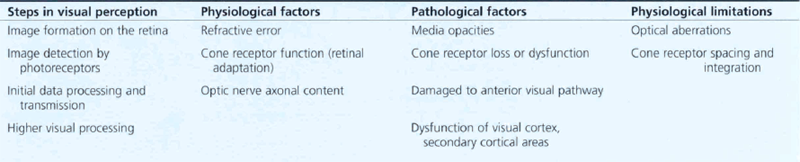
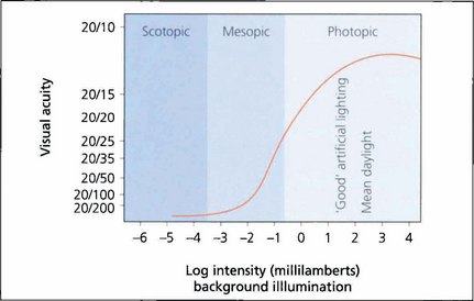
Fig. 1.1 As high-resolution central vision depends on cone receptors any reduction in cone function will greatly compromise acuity. This graph shows visual acuity plotted against background illumination. The best acuity in the scotopic (rod-sensitive) region of the curve is 20/200 (6/60), whereas under photopic (cone-sensitive) conditions acuity can increase to approximately 20/15 (6/5). The curve flattens once optimal conditions are reached and then reduces owing to the effect of dazzle.
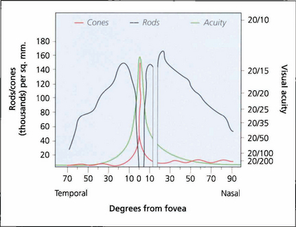
Fig. 1.2 Visual acuity and cone and rod density plotted against degrees from the foveal centre. There are no blue cones at the fovea.
MEASUREMENT OF VISUAL ACUITY
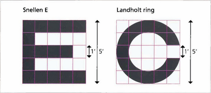
Fig. 1.3 Each individual component of a letter or shape must be resolved to be identified. A letter ‘E’ viewed at the limit of resolution (20/20, 6/6) subtends 5 min of arc, each individual component subtending 1 min. The same principle is used in the construction of the Landholt rings.
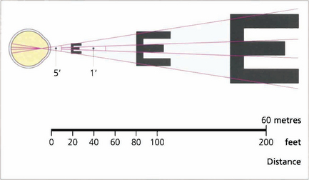
Fig. 1.4 Acuity charts are constructed with rows of letters of different sizes. Letters are constructed so that they subtend the same visual angle at a specified distance of up to 200 feet. Thus the largest letter should be resolvable by a normal eye from 200 feet (60 metres) away and the smallest at 20 feet (6 metres). If the chart is read at 20 feet a normal eye will read all the letters. Any loss of resolution will result in the eye being able to read only larger letters. The test distance is then divided by this line and is expressed as:
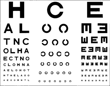
Fig. 1.5 Professor Snellen developed his chart in Utrecht in 1863. The Snellen chart is accepted as the standard chart for clinical practice but it has some problems. Some letters are more legible than others; for example, ‘L’ is easier to read than ‘E’. Patients must also be literate. Modifications to avoid this include Landholt rings where the patient must identify the orientation of a gap or illiterate charts where a cutout letter ‘E’ is matched with the same letter in different orientations.
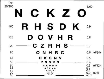
Fig. 1.6 Snellen charts also have the defect of different numbers of letters on each line causing crowding phenomena and nonproportional spacing between letters and lines. Furthermore, the measured range does not extend far enough into low visual acuity ranges. The Bailey–Lovie, Early Treatment Diabetic Retinopathy Study (ETDRS) or LogMAR (log of minimum angle of resolution) chart overcomes these problems. It gives a progressive linear assessment of acuity and has become the standard for clinical research. Each row has five letters with a doubling of the visual angle every three lines. It is read at 4 m and covers Snellen equivalents from 20/200 to 20/10. Each letter read is scored as –0.02 and each row as –0.1 (5×-0.02). Visual acuity is given as the log value of the last complete row read plus –0.02 for each letter read on the row beneath. An acuity of 1.0 equates to 20/200, 0.3 to 20/40, and 0.0 to 20/20. This contrasts with Snellen charts in that the lower the value for visual acuity, the better the vision.

Fig. 1.7 Traditionally near vision testing is done using the appropriate reading correction with a chart of different font sizes. This has, however, no physiological basis and a more scientific method is to use a reduced LogMAR chart such as the MN Read card at a standardized distance and illumination. The text in this chart conforms to LogMAR principles; in addition each paragraph is standardized for length of words, sentences and grammatical complexity. It also allows for reading speed to be measured. Patients need to read at 80 words a minute or better to have functional near vision at that size of print.
©1994, Regents of the University of Minnesota, USA. MNREAD™ 3.1–1/3600.
TESTING ACUITY IN CHILDREN
Visual acuity assessment in children presents particular problems. Good results can be achieved only with time and patience and by selecting the right test for the age of the child. These include qualitative tests such as the child turning to fixate a face or light, suppression of optokinetic nystagmus following rotation or objecting to occlusion of one eye. While semiquantitative measurements are available, for instance picking up ‘hundreds and thousands’ sweets or following small balls quantitative tests are most informative. For infants forced-choice preferential looking or visual evoked potentials (VEPs) can be used; both give different results. Older verbal children can use picture cards (Cardiff cards, Kay’s pictures) and from the age of three may manage matching letter tests (e.g. the Sheridan–Gardiner test; see Ch. 18). Caution is necessary when using Snellen charts with single letters because of the phenomenon of ‘crowding’ – being able to see single letters more easily than rows of letters – which can overestimate true acuity.
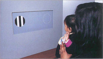
Fig. 1.8 With preferential viewing techniques the child is shown two cards: one has a grating, the other has the same uniform overall luminance. If the child can distinguish the grating, he or she looks at this ‘preferentially’ – presumably because it is more interesting.
By courtesy of Professor A Fielder.
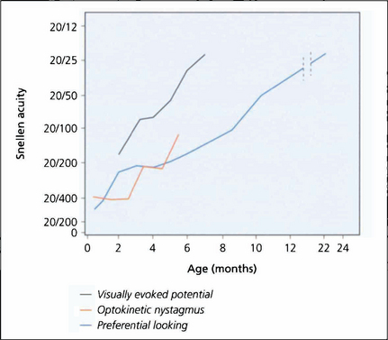
Fig. 1.9 What is known of the development of visual acuity with age depends to some extent on which method of testing was used in studies as VEPs, optokinetic reflexes or preferential looking techniques all give different results. The latter is the most commonly used technique; it shows that infants do not reach adult levels of acuity until 2–3 years of age.
By courtesy of the Editor, Survey of Ophthalmology 1981; 25: 325–332.
PHYSIOLOGICAL LIMITATION OF ACUITY
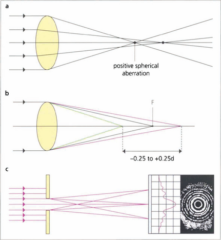
Fig. 1.10 (Top) Spherical aberration. The refractive surfaces of the eye have more effective power at the periphery than at the central paraxial zones. This causes the edge of an image to be blurred by the resulting ‘line spread’. Spherical aberration increases with pupillary dilatation. The eye normally has a positive spherical aberration (see Ch. 11).
WAVEFRONT ANALYSIS
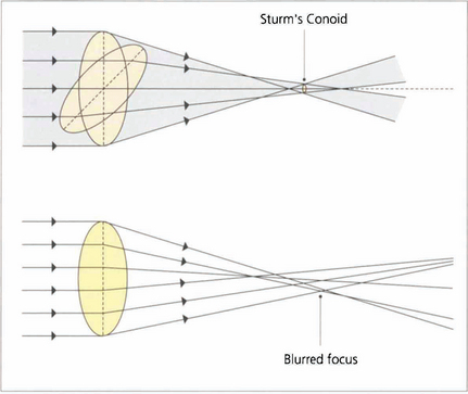
Fig. 1.11 With regular astigmatism, light is brought to focus at two points. Sturm’s conoid is the circle of least confusion that can be brought to focus by a sphero–cylinder combination. With the imperfect optics of the eye light is bought to focus in an irregular manner. This caused by higher-order aberrations which can be demonstrated by wavefront analysis and described mathematically by Zernicke polynomial curve fitting equations.
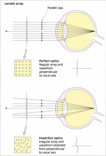
Fig. 1.12 In a perfect optical system rays of light exiting the eye from a spot projected on the fovea should exit the eye parallel to the visual axis with a wavefront perpendicular to the visual axis.
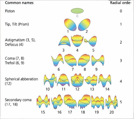
Fig. 1.13 The wavefront deformation from a plane perpendicular to the visual axis can be expressed in terms of a mathematical equation consisting of a series of polynomials. These Zernicke polynomials describe an increasing cascade of aberrations. Low-order aberrations (first and second order: sphere and cylinder) account for more than 90 per cent of refractive error in a normal eye. Third order is coma and fourth order is spherical aberration. Spherical aberration is the clinically most important after sphere and cylinder. Higher orders account for less and less of the aberration. The system becomes extremely complicated as some aberrations can cancel out others; treating one aberration in the absence of all can therefore actually make vision worse.
CONTRAST SENSITIVITY

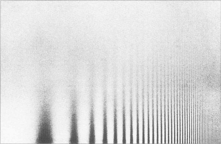
Fig. 1.14 Sine wave gratings can be used to assess contrast sensitivity and spatial frequency simultaneously. The patterns can be generated electronically on a television screen or graphically on a test card or chart. The spatial frequency of the stripes increases along the horizontal axis from left to right (that is, the stripes get thinner and closer together) and the contrast decreases on moving up the vertical axis. As the frequency of the stripes increases to the minimum resolvable acuity (30–40 cycles per second or 1–0.5 min of arc), there is insufficient contrast to distinguish the stripes from the background. As a result the highest resolvable frequencies can be seen only at high contrast (this equates to standard visual acuity tests). Beyond this point the grating appears as uniform greyness. As the spatial frequency decreases there is insufficient contrast to distinguish the stripes from the background illumination.
By courtesy of Mr J W Howe.
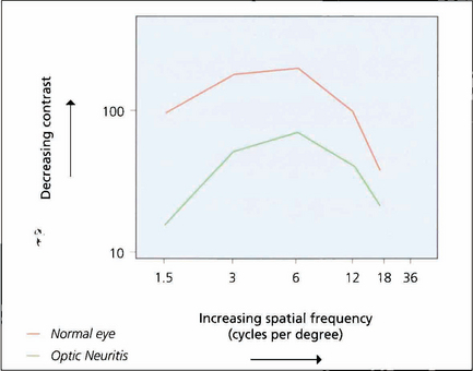
Fig. 1.15 If grating visibility is plotted on a graph, the axes being contrast and spatial frequency, a bell-shaped curve known as a contrast sensitivity curve is formed. At the apex of the curve the subject reaches their highest level of sensitivity at low contrast levels and changes in contrast of 1 per cent or better can be detected. The graph shows the curves of a normal eye compared to the fellow eye with optic neuritis. Although the affected eye has good acuity it will have poorer performance in low-contrast conditions such as poor lighting.
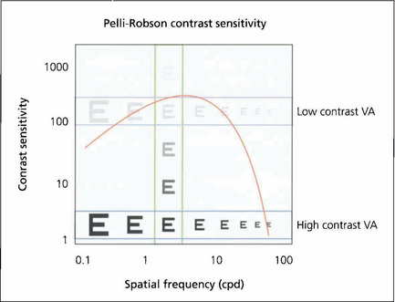
Fig. 1.16 This shows how the different measurements of visual acuity and contrast acuity interrelate. High- and low-contrast visual acuity charts measure a change in spatial frequency at a fixed contrast (horizontal) and the Pelli–Robson chart measures contrast sensitivity at a fixed spatial frequency (vertical).
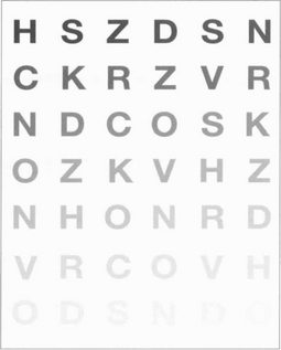
Fig. 1.17 The Pelli–Robson chart is a commonly used method of measuring contrast sensitivity at a set spatial frequency of 6 six cycles per degree. This corresponds both to the spatial frequencies most important in daily life and to the maximum contrast sensitivity of the eye. The chart is viewed at 1 metre under standardized illumination.
COLOUR VISION
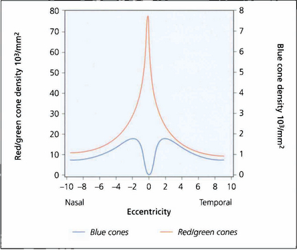
Fig. 1.18 Colour perception is maximal in the centre of the retina but extends out to 25–30° of the visual field. Beyond this, red–green perception disappears and then, in the periphery, all colour perception is absent. There are no blue cones in the fovea and they are less numerous than red–green cones elsewhere in the macula.
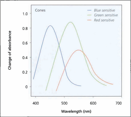
Fig. 1.19 Investigation of the spectral sensitivity curves of the human retina shows peaks at about 440 nm (blue), 540 nm (green) and 570 nm (red). This diagram illustrates the way in which the ranges of wavelength sensitivities of cones overlap; the curves have a gentle slope on the short wavelength side and a rapid fall on the side of long wavelength, that is, towards red.
Adapted from Pyman GA, Sanders L, Goldberg B. Principles and Practice of Ophthalmology. ©1979 Elsevier.
ABNORMAL COLOUR VISION
Abnormal colour vision can either be congenital or acquired; acquired causes include macular and optic nerve damage. Kollner’s rule states that optic nerve disease tends to affect the red–green axis whereas macular damage affects the blue–yellow axis. There are many exceptions to this rule, such as glaucoma and autosomal dominant optic atrophy, which affect the blue–yellow axis; and Stargardt’s disease, which primarily affects the red–green axis. Patients who have abnormal cone populations are not able to match some colours visible to a patient with normal anatomy but have a normal ability within other spectral areas. The most common type of colour deficiency is anomalous trichromacy in which the person has three cone populations but is deficient in one of them. Thus with protanomaly the person is deficient in red cones and needs excess red to match yellow; deuteranomaly requires more green. Dichromats have only two cone systems and thus cannot distinguish certain colours. Protanopes have absence of red cones, deuteranopes green cones. These anomalies are transmitted on the X chromosome and affect about 7 per cent of Caucasian males. Tritanomaly is very rare. These patients have difficulty in distinguishing turquoise blues and greens or yellows and pinks from one another. Achromatopsia is the complete absence of cones. These patients can distinguish colour only in terms of brightness; they have photophobia and poor vision. All patients with congenital colour defects have normal fundi.
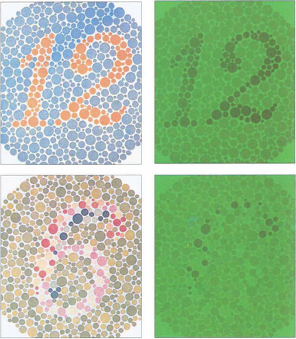
Fig. 1.20 Ishihara plates were originally designed for assessing congenital red–green confusion but are often used clinically to assess colour loss secondary to optic nerve damage. The test consists of plates with a matrix of dots arranged to make either a number or a line that can be traced out. The dots making up the numbers are visible to people with normal red–green colour vision, but are confused with adjacent colours by those who are red–green deficient. The coloured dots are designed to be isochromatic so that the dots making up the letters cannot be perceived by contrast difference alone. A test plate containing the number 12 composed of high-contrast dots is shown at the start to ensure that the subject has sufficient visual acuity to read the numbers. The test plate (a,b) and a trial plate (c,d) are illustrated, with and without a green filter. With the green filter, the test number almost disappears, but the trial plate number is still easily visible as the plate can be perceived by contrast rather than colour discrimination.
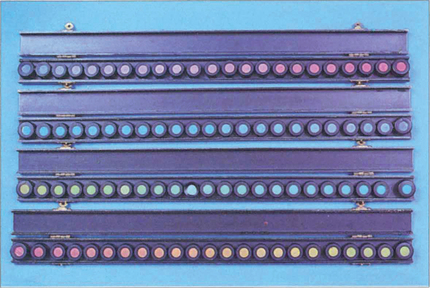
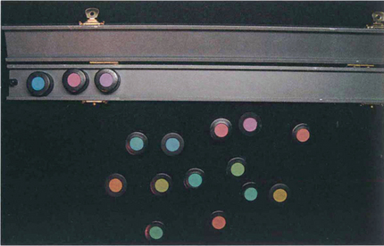
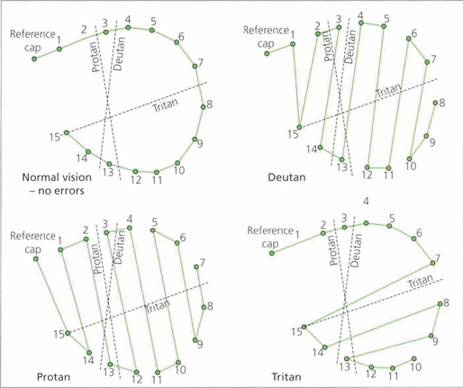
Fig. 1.21 Despite its name, the Farnsworth–Munsell 100 hue test actually consists of 84 coloured tiles arranged in four separate trays. In the test the difference between the tiles is graded so that there is one unit of ‘just noticeable difference’ between them. Each of the four trays covers a different range of the colour spectrum. Trays of tiles are taken one at a time and jumbled. The patient then views these under a standard white light and rearranges the tiles in chromatic order between the two reference tiles placed at each end of the tray. The misalignment of the tiles from their correct position in the chromatic series is then scored and marked on a standard chart; the greater the displacement, the higher the score. The test is considerably faster when using computerized reading and plotting.
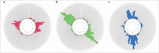
Fig. 1.22 In a normal person only one or two tiles would be misplaced, and the score sheet would appear as a small circle. In the different colour anomalies, however, the chart becomes distorted along a particular axis. The axis of distortion is typical for a particular colour deficiency; examples of the axis for protanomaly (a), deuteranomaly (b), and tritanomaly (c) are shown. Patients with nonspecific acquired colour defects usually make errors in all parts of the wheel.
VISUAL FIELD TESTS
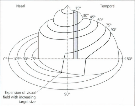
Fig. 1.25 The plot of the visual field isopters can be represented in a three-dimensional form called Traquair’s Island, in which the isopters appear as contour lines on the island. The height of any point on the island is proportional to the sensitivity of stimulus detection at that point and thus is inversely proportional to the threshold. The topography of the island is not static but varies with retinal adaptation. Under mesopic conditions, the gradient of sensitivity away from the central areas is much more gentle than under photopic conditions, where the peripheral retina is desensitized and foveal function is more acute. For this reason, it is important that comparisons of the visual field are made under standardized conditions of retinal adaptation.
MEASURING VISUAL FIELDS
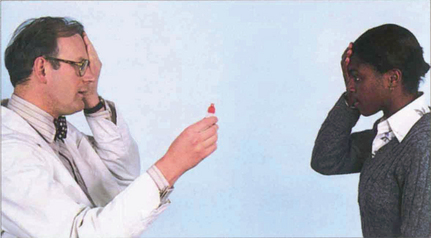
Fig. 1.26 The simplest way to test the visual field is a confrontation technique. The examiner sits opposite the patient at a distance of approximately 1 m. The patient and examiner cover opposite eyes with their palms so that the uncovered eyes have mutually congruent fields. The examiner then introduces a test target into the field (fingers, hand, red bottle cap) until the target is perceived by the patient (kinetic perimetry). The patient’s and examiner’s fields should be congruent, so the presence of a defect is noted by the absent patient response when the object is visible in the examiner’s field. A red target is especially useful for detecting early neurological defects in the central 30° of the field. This is because the retrobulbar pathways are particularly sensitive to red, being concerned mainly with macular vision. If the patient is asked to compare the quality of colour between quadrants (static perimetry) very early defects, such as a bitemporal hemianopia, can be detected subjectively. With practice, a confrontation field can be obtained from almost any patient and produces helpful localizing information.
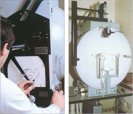
Fig. 1.27 The Goldmann perimeter is usually used for kinetic perimetry but can be adapted for some basic static perimetry. It consists of a hemispherical bowl that is uniformly illuminated and on to which target lights of varying size and brightness are projected. Target size, brightness, colour, background illumination and fixation are all controlled. The patient sits at the machine with the eye to be tested fixed on the centre of the hemisphere. Fixation is checked by an observation telescope mounted at the central fixation point. The target lights are then introduced by the projector into the visual field of the patient while a pantograph arm moves across a standard recording chart at the rear. As the patient signals perception of the target the examiner marks the chart and eventually plots the isopter to the particular target. The test is usually undertaken at several isopters of target size and brightness, thus producing a kinetic field that demonstrates the area and density of field loss. A static assessment can be made by flashing the target light within the appropriate isopter. Goldmann fields have the disadvantage of being somewhat examiner dependent but they do assess the full field area making them useful for assessment of neurological deficits.
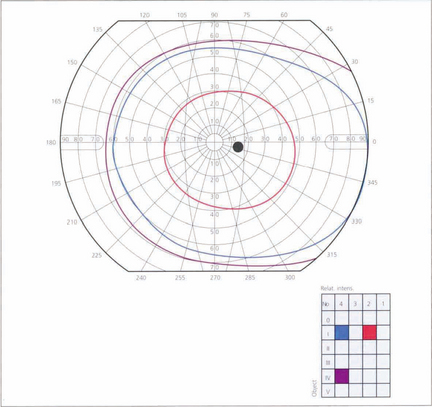
Fig. 1.28 A typical visual field as plotted on a Goldmann perimeter. The visual field, which is marked off in degrees from the fovea, is not circular but displaced laterally and downwards. The upper and medial limits are approximately 60°, the temporal 100° and the inferior 75°. In the temporal field the exit of the optic nerve is marked by the blind spot, 5.5° in height and 5° wide, the centre being about 15° from the centre of foveal fixation. The prominence of the brow and the nose may cause artefacts in the nasal and superior visual field that the examiner must be aware of and able to correct.
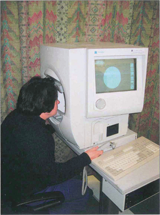
Fig. 1.29 The most commonly used computer-assisted static perimeter is the Humphrey analyser, shown here. Static targets of fixed size but variable intensity are presented randomly at different retinal coordinates within a bowl perimeter of constant photopic background illumination (21.5 asb). These coordinates have been selected for their discriminatory potential in glaucoma. Fixation is automatically monitored and displayed on a television screen to the side. Throughout the procedure the software program checks and rechecks that fixation is maintained and scores how well the patient fixates. To test for false-positive results the stimulus is withheld when the machine audibly indicates stimulus presentation. False-negative findings are assessed by re-examining a number of tested areas with a suprathreshold stimulus. The duration of the test depends on the number of repetitions at each point and the speed of the patient’s response. To perform well the patient needs to be familiar with the test – a learning curve is often demonstrated. The Octopus machine is another computer-assisted static perimeter using a mesopic background illumination (4 asb).
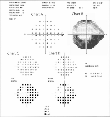
Fig. 1.30 Computer printout from a Humphrey visual field analyser showing the location and sensitivity of the 54 tested retinal loci in the 24-2 program. Chart A represents the actual retinal threshold at each locus in decibels. Chart B shows this as a grey scale for rapid interpretation. Chart C shows the total deviation. This is the difference at each point from an age-matched control; the lower chart converts this to a statistical probability. Chart D adjusts this to compensate for any generalized depression across the field (e.g. from cataract or miosis), thereby defining focal loss more clearly. Average numerical ‘global indices’ for these deviations are also given as mean deviation (MD) and pattern standard deviation (PSD). In addition, reliability indices are given on the printout. These are fixation losses, false positives (trigger-happy patient) and false negatives (inattentive patient). This is assessed by measuring the threshold twice at ten predetermined points.
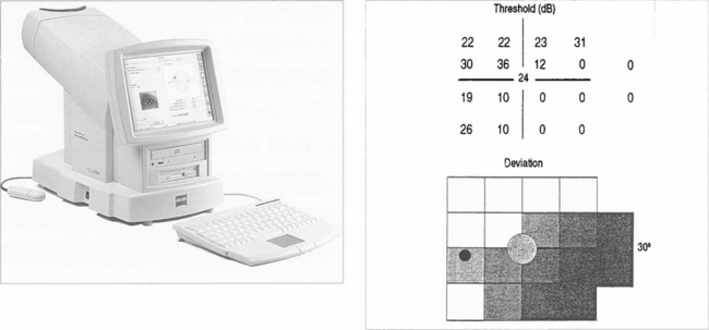
Fig. 1.31 Glaucoma has been shown preferentially to affect the large-diameter optic nerve axons (magnocellular pathway). Several new tests are designed to exploit this and have considerable clinical potential. Frequency doubling perimetry projects a low frequency (1 cpd) sine wave grating into a sector of the retina. The grating is moved at high temporal frequency until the patient gets the sensation that the frequency of the grating has doubled (i.e. there are twice as many bands); this is the endpoint. The test is rapid and sensitive, can be done in room light, and patients prefer it to conventional perimetry. Another new test is SWAP (shortwave automated perimetry) which uses a blue target on a yellow background. This test is very sensitive in detecting glaucoma defects but is affected by cataract.
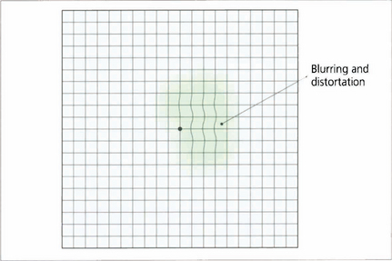
Fig. 1.32 The Amsler grid is a field test that assesses the central 10° of vision qualitatively. It is an effective and rapid method for detecting macular abnormalities that cause blurring or distortion. The test is monocular. The patient holds the grid 25–30 cm away, fixing on the central dot and draws around the area of abnormality. Sequential grids are very useful to follow changes.
OCULAR EXAMINATION
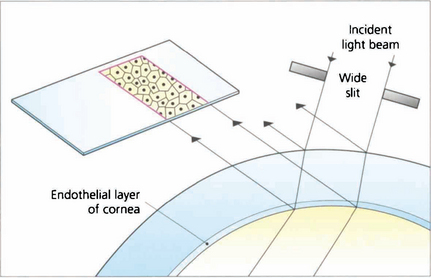
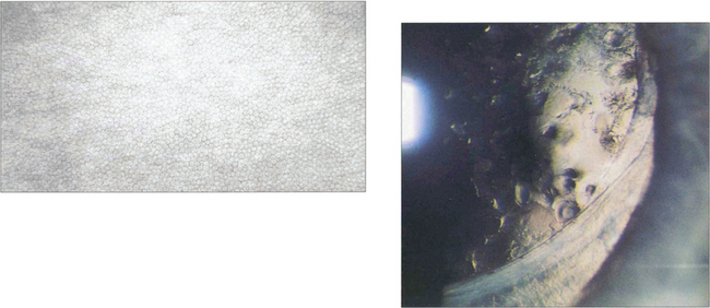
SPECULAR MICROSCOPY
CORNEAL TOPOGRAPHY AND KERATOMETRY

Fig. 1.35 Corneal topography. The photograph of the reflected image and its distortions are analysed by computer to produce a topographical map of the anterior corneal surface giving quantitative information on the corneal curvature. From this, corneal astigmatism and its meridians can be calculated.
©1995–2002 Bausch & Lomb Inc.

Fig. 1.36 Topographic printouts are colour coded. By convention steep areas are coloured red and flat areas blue although the actual dioptric values for each colour are not standardised between instruments. Most normal corneas remain within the yellow-green spectrum of the scale. Common patterns seen include a bow tie pattern in astigmatism and a central steep island in keratoconus (see Chapter 6). This eye has an old scar inferio-nasally. The pachymetry map shows this area is thinned. Topography shows this area is slightly ectatic with a steeper curvature causing irregular astigmatism.
©1995–2002 Bausch & Lomb Inc.
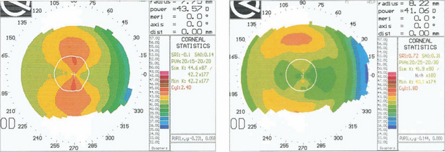
Fig. 1.37 This technology is essential in the assessment of refractive corneal surgery. These charts show a cornea before excimer laser ablation (left). The isopters are graded in 1D steps and show with the rule astigmatism of 2.4D. After photoablation (right), the astigmatism has been reduced to 1.8D with the rule and there has been a reduction of myopia of 2.5D.
By courtesy of Mr D O’Brart.
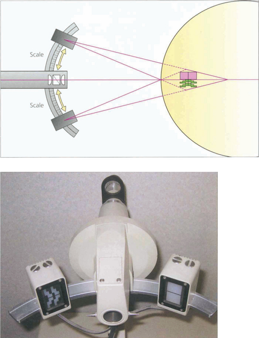
Fig. 1.38 Corneal curvature is routinely measured before cataract surgery to calculate intraocular lens power. Although this information can be obtained from detailed topography only the curvature of the central 3 mm of cornea is important for this and this can be obtained from a simplified topographic technique or by manual keratometry. The spherical power in the axis of the two regular meridians can easily be measured using a basic keratometer of which there are two types (Schiotz and Helmholtz). The former uses an object of varying size and the latter an image of varying size.
GONIOSCOPY
Gonioscopy is the visualization of the angle of the anterior chamber.
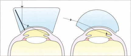
Fig. 1.39 The optics of indirect and direct gonioscopy are illustrated. Direct gonioscopes (e.g. Barkan) provide an erect view of the eye and are used for surgical goniotomy for buphthalmos. Indirect gonioscopy (e.g. with a Goldmann or Zeiss lens) produces a mirror image of the opposite angle and is used with a slit lamp for diagnostic purposes or laser goniotomy. It can be combined with corneal depression (indentation gonioscopy) to assess whether the angle can be opened by the displaced aqueous. Such indentation gonioscopy is invaluable in assessing primary angle-closure glaucoma.
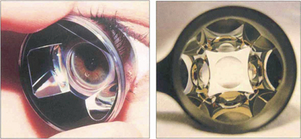
Fig. 1.40 The Goldmann indirect gonioscopy lens is a solid perspex contact lens within which is mounted a small steep mirror. The lens requires a coupling medium for use, such as saline or hypromellose, as its curvature is steeper than that of the cornea. The full circumference of the angle can be inspected by rotating the contact lens on the surface of the eye. Lenses such as the Zeiss 4 mirror goniolens have a shallower radius of curvature and hence do not require fluid between the lens and the cornea; however, this makes corneal wrinkling more likely. The additional mirrors eliminate the need to rotate the lens; such lenses will also easily indent the cornea for indentation gonioscopy.
Left image by courtesy of Mr B Dong.
TONOMETRY
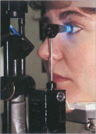
Fig. 1.41 The Goldmann tonometer has an applanating surface of 3.06 mm2, at which the effect of surface tension cancels out the rigidity of the cornea. It indents the eye less than 0.2 mm, displaces 0.5 ml of aqueous and increases the IOP by approximately 3 per cent which is not clinically significant. The applanation head has a clear centre that incorporates a prismatic doubling device. Before use the corneal epithelium is anaesthetized and stained with fluorescein to identify the tear meniscus around the applanating head. The prism is illuminated obliquely by the slit lamp with the cobalt blue filter and the cornea is viewed coaxially through the applanation head which is then gently brought to rest on the surface of the cornea. The force applanating the cornea is increased by revolving a graduated wheel at the base of the instrument, calibrated in millimetres of mercury.
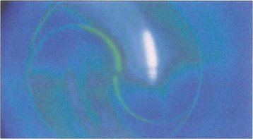
Fig. 1.42 This shows the endpoint at which the IOP is measured. The split image of the tear film meniscus can be seen around the tonometer head, outlined by the semicircular fluorescein rings with the edges just overlapping. If the pressure on the tonometer head is too low, the resulting applanation area is small and the split rings do not overlap; if it is too high, they overlap by more than the thickness of the meniscus.
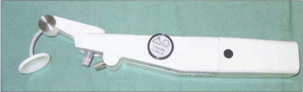
Fig. 1.43 The Perkins tonometer is a hand-held variant that employs a Goldmann prism. The body rests on the patient’s forehead and the fluorescein rings are viewed through a convex lens aligned with the prism head. It is often used for assessing IOP in anaesthetized children or patients who cannot sit at a slit lamp.
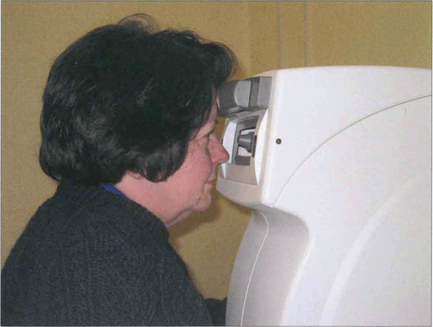
Fig. 1.44 Noncontact applanation tonometers use a puff of air to deform the cornea and measure the time taken to produce a set amount of corneal flattening. This time is proportional to the IOP. The reliability of this type of tonometer is reduced in higher pressure ranges but it has the advantage of no contact with the eye, thus preventing any risk of cross-infection and obviating the need for topical anaesthesia making it ideal as a screening device in optometric practice.
IMAGING THE GLOBE AND ORBIT
OPHTHALMOSCOPY
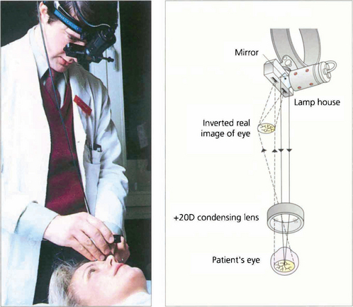
Fig. 1.45 The indirect ophthalmoscope uses a condensing lens to gather the light reflected from the subject’s retina, forming a real inverted image of the retina between the examiner and the subject. Light is derived from a source on the examiner’s headpiece that is directed into the patient’s eye by an adjacent adjustable mirror. As the light source is further away from the patient’s eye than with the direct ophthalmoscope, the patient’s pupils must be dilated to allow a sufficient field of illumination. The image that is formed is viewed through an eyepiece on the examiner’s headpiece; this narrows the examiner’s true pupillary distance and allows binocular viewing and stereopsis. The examiner is standing behind the patient so that the inverted image that is seen corresponds to the normal erect appearance.
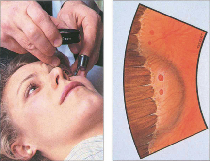
Fig. 1.46 Further detail, especially at the retinal periphery, can be seen by using an indentor to push peripheral retinal areas into the instrument’s field of view. Movement of the indentor induces dynamic forces and helps to highlight pathology such as shallow retinal separations or tears.
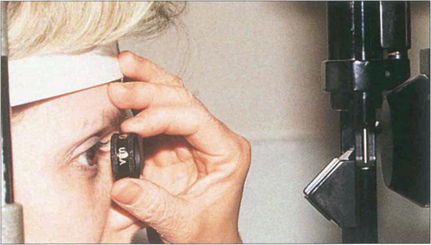
Fig. 1.47 Slit lamp stereoscopic biomicroscopy using an aspheric lens and the same principle as indirect ophthalmoscopy has become the technique of choice for standard clinical fundus examination as it has the advantages of bright illumination, stereopsis and high magnification. A wide variety of lenses are available which have differences in magnification and field of view.
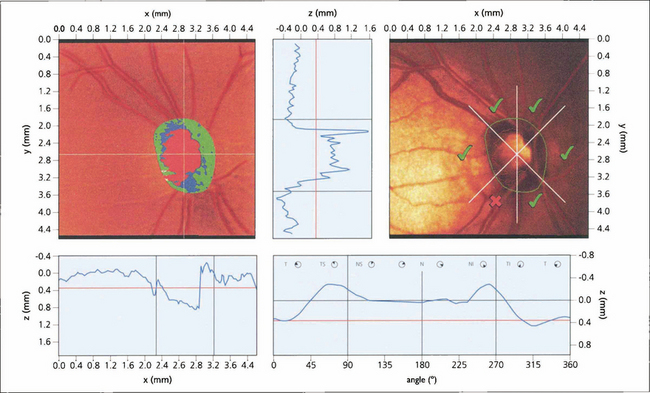
Fig. 1.48 The scanning laser ophthalmoscope (SLO) uses narrow, collimated, low-power He–Ne laser light to illuminate the retinal surface or optic nerve head. These systems have the advantage of producing real-time fundal images that can be analysed and stored digitally. In a basic system a broad beam of low-intensity light is reflected from the fundus and detected and processed to give an image of the illuminated area. More sophisticated systems use point-by-point raster scanning over a region of interest and, in confocal scanning laser tomography, imaging can be conducted in different optical planes to allow subsequent three-dimensional analysis of a structure. Introducing filters and confocal diaphragms in the path of the laser allows the nature of resulting image data to be controlled very precisely so that unwanted reflections or scattered light can be removed to give clear pictures in conditions otherwise considered challenging for conventional photography and to allow imaging through undilated pupils. For example, introducing an ellipsometer allows the amount of reflected polarized light from the eye to be measured; different filters allow fluorescein, indocyanine green (ICG) or autofluoresence to be imaged. SLOs have wide applications in clinical research and may well come into clinical practice to monitor optic disc changes in glaucoma (see Ch. 7).
OPTICAL COHERENCE TOMOGRAPHY (OCT)
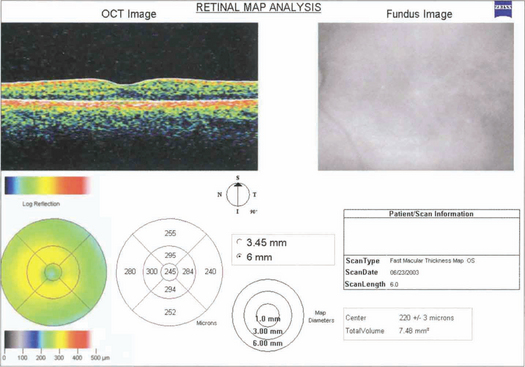
OCT obtains images by using back scattering of light in a way analogous to ultrasound B scanning but as the wavelength of light is shorter the resolution is much higher. It uses a low-coherence infrared beam that is split into a probe beam incident on the retina and an external reference beam directed on to a mirror held at a known distance. The incident beam is reflected by different interfaces within the retina and retinal pigment epithelium but penetration of deeper tissues is very limited. The two reflected beams are then recombined and their interference is measured producing a depth-specific interference signal with a longitudinal resolution corresponding to depth and an amplitude corresponding to the tissue reflectivity at that point. The degree of reflectivity is displayed in false colour giving an ‘anatomical’ display. Cross-sectional imaging is achieved by combining a sequence of A-scan profiles across the retina, analogous to ultrasound B scans. OCT has become essential in the clinical evaluation of macular pathology such as macular holes, cystoid oedema, pigment epithelial detachment and preretinal membranes, and the demonstration of vitreous traction (see Ch. 12). It is less useful for investigation of subretinal pathology such as neovascular membranes. Future developments of OCT show great potential for measuring optic disc cupping and nerve fibre layer thickness in glaucoma. Recently a new OCT with a wavelength of 1310 mm has been developed for anterior segment imaging which is likely to be of great benefit in signing the anterior chamber for phakic intraocular lenses. This wavelength is reflected by transparent ocular tissues such as the cornea and lens.
ULTRASONOGRAPHY
Ultrasound is mainly used to visualize intraocular structures through opaque media or to measure intraocular dimensions for intraocular lens biometry or to assess tumour size. It can also be used to visualize some orbital structures but the technique is difficult and operator dependent. Ultrasound is reflected at changes in tissue density. Images of the eye can be obtained in one or two dimensions (A or B scan). A-scan images provide a linear view along one axis and are used to measure lengths within the eye; B-scan ultrasonography uses A scans placed together to form a two-dimensional picture. It is a rapid, easy method of imaging intraocular contents and also allows dynamic examination, for example, of retinal detachment. High-frequency probes (50 MHz) give much higher resolution but poor tissue penetration; they are very useful for imaging anterior chamber detail (see Ch. 7)
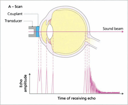
Fig. 1.50 The scanning probe consists of an ultrasound emitter and a transducer that detects signals echoed (reflected) from tissue interfaces; echo amplitude is proportional to the acoustic mismatch between adjacent tissues. In a normal eye peaks can be identified from the corneal endothelium, anterior and posterior lens surfaces, and the retina. The A-scan mode is used routinely to measure axial length; to do this the probe is placed directly on the patient’s anaesthetized cornea. Distance calculations are derived from the speed of sound in each media and settings should be adjusted when an eye has cataract or is aphakic, pseudophakic or oil-filled.
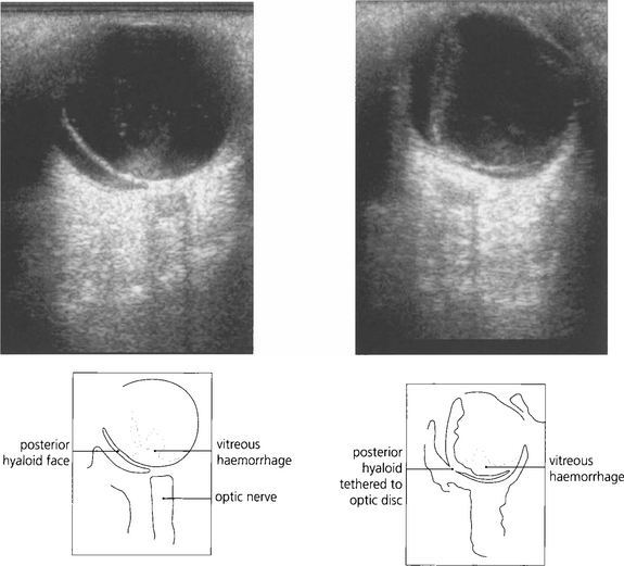
Fig. 1.51 A B scan is a cross-sectional image that is formed when the eye is scanned in A mode across several planes. The optic nerve looks dark because its substance is homogeneous and of low reflectance and therefore lacks tissue interfaces from which significant reflectivity can arise. For dynamic images, the eye should be scanned in a horizontal and vertical plane, with the eye stationary and moving (up and down and from side to side). The probe carries a marker that orients the examiner to the plane of imaging in the eye. Shown here are two images of the same eye with the patient looking left (top) and then right (bottom). There is a vitreous haemorrhage (high signal). The detached and collapsed gel is suspended from its basal attachments and moves with the eye.
By courtesy of Mr E Herbert.
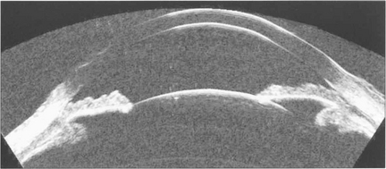
Fig. 1.52 High frequency probes (50 MHz) give very much higher resolution at the expense of poor tissue penetration. It is very useful for imaging anterior chamber detail such as angle pathology, (see Chapter 7), ciliary body tumours or sizing AC dimensions for anterior chamber IOLs.
By courtesy of Dr D Reinstein.
COMPUTED TOMOGRAPHY (CT)
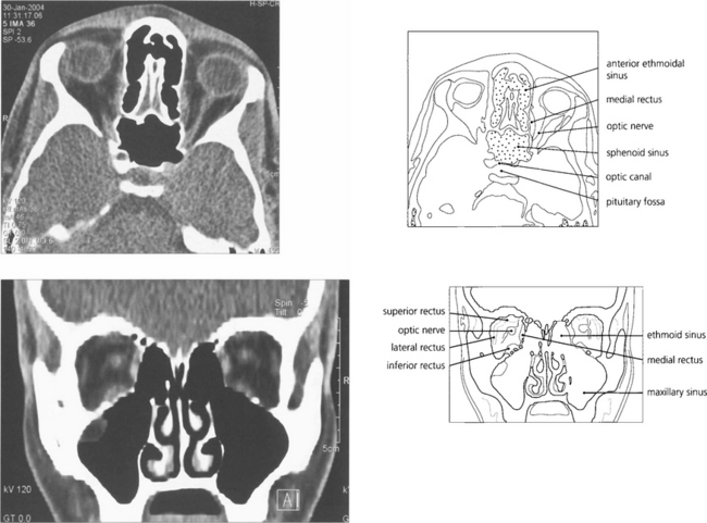
Fig. 1.53 Axial and coronal CT scans of the orbit demonstrating the orbit and its contents. Coronal views are extremely useful for assessing intraorbital lesions as they avoid the partial volume effect of axial scans with lesions in the superior or inferior orbit and are easier and safer to interpret. Contrast can be given for further enhancement of vascular lesions.
MAGNETIC RESONANCE IMAGING (MRI)
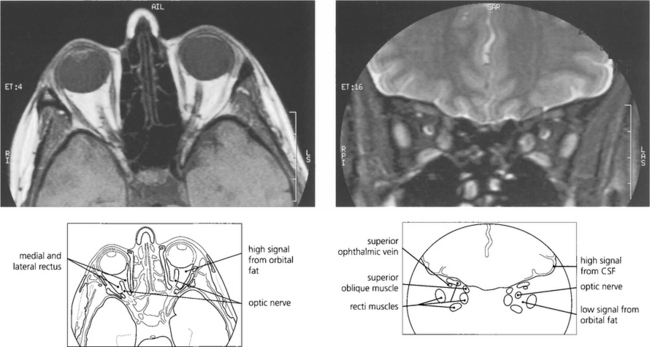
Fig. 1.54 (Left) The retrobulbar orbital fat has a high signal T1 MRI sometimes making it difficult to visualize orbital pathology. By using specialized sequences the fat signal can be suppressed giving much better visualization (right). This is particularly useful in identifying optic nerve pathology.
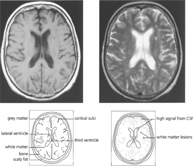
Fig. 1.55 T1-weighted scans have a low CSF signal and provide excellent anatomical detail. With T2 weighting the anatomical detail is less clear but pathological lesions are frequently demonstrated more easily. This patient has white matter lesions in the left cerebral hemisphere compatible with demyelination in a young adult or small vessel vascular disease in the elderly.
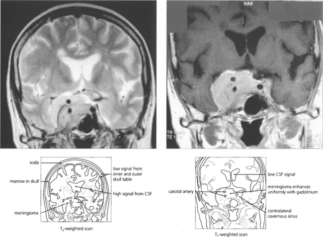
Fig. 1.56 Intravenous gadolinium shows breakdown of the blood–brain barrier in a way analogous to CT scanning with IV contrast enhancement and is particularly useful in demonstrating pathology and the extent of a lesion and surrounding oedema. This patient has a cavernous sinus meningioma. The lesion shows typical uniform enhancement with gadolinium and its anatomical extent can be seen much more easily. It surrounds the ipsilateral carotid artery and spreads through the pituitary fossa to the contralateral sinus.
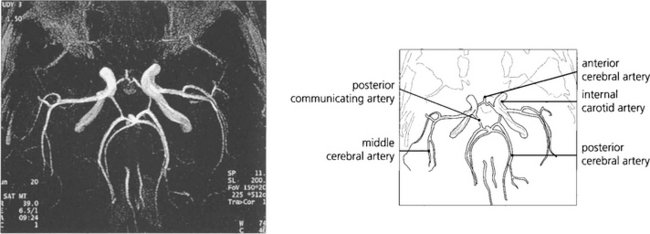
Fig. 1.57 Magnetic resonance angiography (MRA) has now largely superseded other forms of cerebral angiography as a diagnostic technique as it is noninvasive and therefore avoids the risk of traditional angiography. This image shows the vascular anatomy of the circle of Willis.
With permission from Yanoff et al (eds) Ophthalomology © 2003 Elsevier Inc.
ELECTRICAL TESTS OF RETINAL FUNCTION
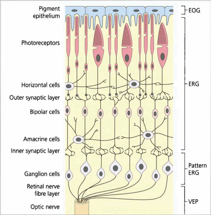
Fig. 1.58 The regions of the retina responsible for generating the various electrical potentials. The EOG is generated by the retinal pigment epithelium–photoreceptor complex and photoreceptors. The ERG is a complex potential, reflecting photoreceptor and inner nuclear layer function. The PERG is partially generated in the ganglion cells (N95 component), providing objective data on ganglion cell function and partially in the more distal retina (some of the P50 component). However, much of the P50 component is driven by the macular photoreceptors and so provides an objective index of macular function. The VEP provides objective assessment of the retrobulbar and intracranial pathways.
DARK ADAPTATION
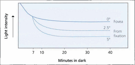
Fig. 1.59 Dark adaptation curve. Threshold light intensity is plotted against time following bleaching by a bright flash and shows that the retina becomes more sensitive as rhodopsia is regenerated. The three lines indicate different retinal thresholds at 0, 2.5 and 5° from the fovea and show that dark adaptation increases eccentrically from the fovea as the population of rods increases. The cone–rod threshold at 7 min is shown.
ELECTRO-OCULOGRAPHY (EOG)
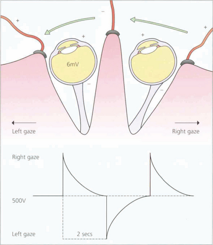
Fig. 1.60 This potential can be measured by surface electrodes placed on the medial and lateral canthi. The patient is asked to make horizontal eye movements between two fixation lights that alternate from right to left, 15° either side of centre, enabling constant 30° excursions to be made. Movement of the cornea to or away from the electrodes thus induces an electrical potential which is amplified and recorded. During a period of scotopic adaptation, the potential falls to a minimum – the dark trough – after approximately 12 min of dark adaptation. The potential reaches a maximum after approximately 8–10 min of photopic adaptation, reflecting progressive depolarization of the basal membrane of the retinal pigment epithelium.
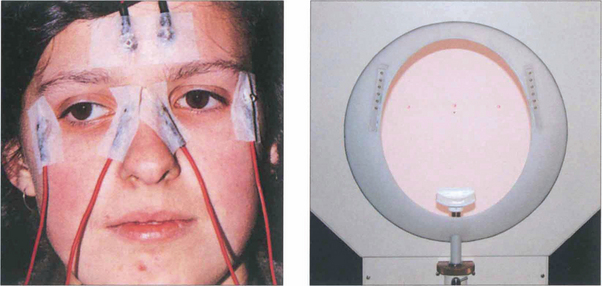
Fig. 1.61 Clinically the test is performed with dilated pupils using a Ganzfeld bowl, which produces uniform retinal illumination during the photopic phase. The patient sits with their chin on the chin rest. During EOG recording only the central fixation light is illuminated. On either side (15° from centre) are the two LEDs that the patient fixates alternately during the test. Below the central fixation light there is a small infrared camera for monitoring the patient. The potential is measured during scotopic adaptation for 20 min, during which time the dark trough occurs. The illumination is then increased to photopic levels and recordings are continued for a further 15 min or until the light peak has been reached. The ratio of light peak to the dark trough should exceed 175 per cent in normals. A reduced EOG light rise indicates dysfunction at the level of the retinal pigment epithelium–photoreceptor complex. Accurate assessment of the EOG requires the patient to be able to make accurate and replicable horizontal eye movements and although readings are not affected by opacities in the ocular media dense cataracts prevent compliance as the patient cannot see the fixation lights.
By courtesy Mr C R Hogg.
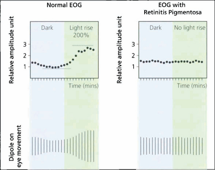
Fig. 1.62 Typical tracings of a normal patient compared with those from a patient with retinitis pigmentosa. There is neither an EOG dark trough nor a light rise in the patient with retinitis pigmentosa. The test is particularly useful in the diagnosis of Best’s vitelliform macular dystrophy (see Ch. 16).
ELECTRORETINOGRAPHY
A standardized bright flash is given. The response to this flash under scotopic conditions with a fully dilated pupil, is the maximal or mixed response (see Fig. 1.64). This response, perhaps regarded by many as the ‘typical’ ERG is dominated by rod-driven activity. The initial negative component is known as the a-wave, approximately the first 10 ms of which reflects photoreceptor hyperpolarization; the A-wave slope reflects the kinetics of phototransduction. The larger positive B-wave which follows the A-wave is generated after phototransduction in relation to ‘ON’ bipolar cell depolarization. The oscillatory potentials, the small wavelets seen on the B-wave, probably relate to activity in the amacrine cells. When the standard flash is reduced by 2.5 log units a rod-specific response is obtained consisting purely of the inner nuclear derived B-wave; at these low luminance levels, even under scotopic adaptation, there is insufficient photoactivation to record an A-wave (see Fig 1.64).
The ISCEV standard rod-specific response is generally the most sensitive detector of rod system dysfunction. However, this response (the rod-specific B-wave) is generated in the inner nuclear layer and thus does not allow distinction between photoreceptor dysfunction and postphototransduction dys-function. This distinction is better seen in the bright-flash ERG response where significant a-wave reduction indicates photoreceptor dysfunction (see Fig. 1.65), such as occurs in genetically determined photoreceptor degenerations. If the site of dysfunction is postphototransduction there may be a normal a-wave with selective B-wave reduction (the so-called negative or electronegative waveform; see Fig. 1.65). Among the diseases that lead to a ‘negative’ ERG are X-linked congenital stationary night blindness, X-linked juvenile retinoschisis, central retinal artery occlusion and quinine toxicity.
Cone-specific ERGs are recorded when the retina is stimulated under conditions of photopic adaptation. This is done by increasing the background illumination to suppress the rods and using both single-flash and 30-Hz flicker stimulation. At 30 Hz the poor temporal resolution of the rod system, in addition to the presence of the rod-suppressing background, enables a cone-specific waveform to be recorded (see Fig. 1.64) illumination. It is a more sensitive measure of cone dysfunction but is generated at an inner retinal level. In contrast, the single-flash cone response gives better localization within the retina. Although there is a contribution of the hyperpolarizing (OFF) bipolar cells to shaping the photopic a-wave, the cone photoreceptors probably also contribute to the generation of this component. The cone b-wave reflects postphototransduction activity. There is no significant retinal ganglion cell contribution to the clinical (flash) ERG.
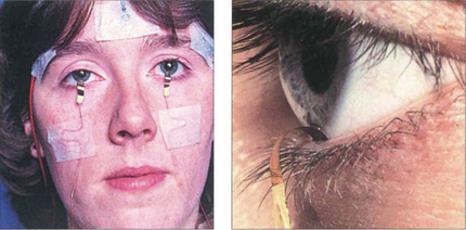
Fig. 1.63 The main recording electrode for the ERG is corneal, and is often a contact lens electrode, but gold foil and loop electrodes in the fornix are also acceptable and in common use. The reference electrodes should be positioned at the outer canthi. Corneal electrodes that do not alter the optics of the eye can be used for both full-field and pattern ERG recording. The gold-foil electrode is a thin layer of gold leaf with a mylar base placed over the lower eyelid so that it is in contact with the lower limbus of the cornea; it is important that it does not touch the skin of the lower eyelid. Surface-active electrodes can be used in unsedated infants to give adequate but limited recordings; ERGs can also be recorded under general anaesthesia.
PATTERN ELECTRORETINOGRAPHY
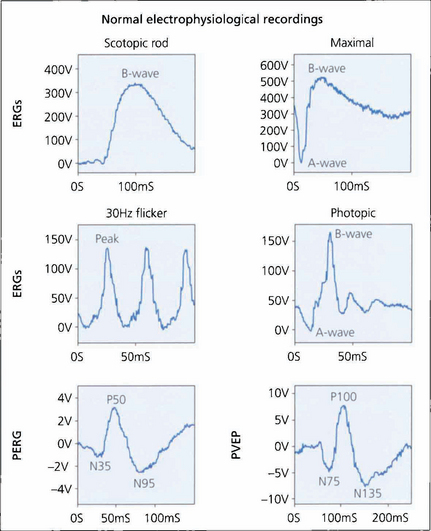
Fig. 1.64 Typical normal electrodiagnostic waveforms. A bright white light (of standardized intensity) in a dark-adapted eye gives a mixed rod–cone response with a prominent A-wave although this response is dominated by rod function. The first 10–12 ms of the A-wave reflects the kinetics of phototransduction. Amplitude and implicit time of the A- and B-waves are measured. Note the presence of the amacrine cell-related oscillatory potentials on the B-wave which can be enhanced by selective filtering. A dim flash in a fully dark-adapted eye gives a scotopic rod-specific response consisting of a positive B-wave with no recordable A-wave. Amplitude and implicit time (the time to peak) of the b-wave peak are measured. Cone function is assessed under photopic conditions using a rod-suppressing background with a 30-Hz white light, which gives a cone-derived flicker response, or single-flash stimulation. The flicker response and A- and B-wave amplitude and implicit times are measured for the photopic single-flash response. Measurement of the PERG focuses on the amplitude and timing of the P50 component and the amplitude of the N95 component. Both components are measured ‘peak-to-peak’. Pattern visual evoked potential measurement concentrates on the implicit time (often referred to as latency) and amplitude of the P100 peak.
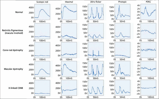
Fig. 1.65 Examples of ERGs to show the ability of the ERG both to separate rod and cone system function and to ascertain the degree of dysfunction. Typical normal findings are shown for comparison. In the patient with retinitis pigmentosa, the rod-specific ERG B-wave is profoundly subnormal. The marked reduction in the maximal A-wave response confirms that this is related to photoreceptor dysfunction. Cone single-flash and flicker ERGs both show amplitude and implicit time abnormalities but the changes are less severe than those in the rod system. Thus, the patient has a rod–cone dystrophy. The subnormal PERG confirms macular involvement.
VISUAL EVOKED POTENTIAL
The visual evoked potential (VEP) is the electrical response of the visual cortex to visual stimulation and is recorded using posteriorly situated scalp electrodes. It is extracted from the spontaneous higher-voltage background activity of the brain, the electroencephalogram, by using repetitive stimulation and computerized signal averaging. The VEP, like the PERG, varies with stimulus and recording parameters. The normal-pattern VEP response to a slowly (approximately 2 cycles per second) reversing black and white chequerboard in constant luminance contains a prominent positive peak at about 100 ms; this is known as P100 (see Fig. 1.64), and its amplitude and latency are measured. This pattern-reversal VEP is most commonly used in routine clinical practice.
VEPs are particularly useful for detecting and diagnosing optic nerve disease. Optic nerve demyelination profoundly delays the VEP and this is almost invariable following a clinical episode of optic neuritis and may also be seen in subclinical disease. Ischaemic optic neuropathy tends to affect amplitude rather than latency. Although optic nerve disease often results in VEP delay, VEP delays also commonly occur with macular dysfunction so that the PERG may be needed to distinguish accurately between optic nerve and macular disease. The VEP can also be useful in the assessment of chiasmal function by comparing responses from the nasal and temporal hemifields. The VEP to both flash (in younger children) and pattern appearance (in older patients) is the investigation of choice in identifying the abnormal intracranial misrouting of albinism. VEPs also have a valuable role in the diagnosis of nonorganic visual loss, where they can objectively demonstrate normal function in the presence of symptoms that suggest otherwise.
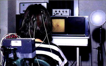
Fig. 1.66 The VEP is recorded by placing electrodes on the scalp (electrodes placed on the right occiput record signals from the left occipital cortex). Repeated responses to the reversing chequerboard stimulus are recorded and averaged. It is important to ensure the patient is fixating on the pattern because loss of fixation can cause artefacts; this is especially important in patients suspected of having nonorganic visual loss.
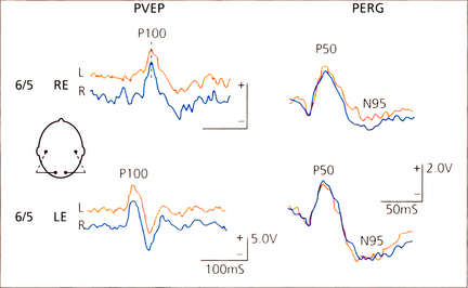
Fig. 1.67 Pattern visual evoked potentials (PVEPs) and PERG in a patient with recovered retrobulbar neuritis. Despite clinical recovery to normal visual acuity the PVEP P100 component is delayed to 135 ms in the affected right eye. Note the symmetical PERG P50 component in both eyes but selective reduction of the N95 component in the right-eye PERG which is due to degeneration of the retinal ganglion cells following the episode of optic nerve demyelination.
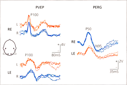
Fig. 1.68 PVEP and PERG in a patient with left inflammatory maculopathy. The P100 component of the VEP is delayed and broadened in the affected left eye and the PERG P50 component is reduced and delayed. Compare this PERG abnormality with the N95 abnormality consequent upon retrograde degeneration to the retinal ganglion cells in the patient with retrobulbar neuritis in Fig. 1.67.