Ocular Biometry

Published on 08/03/2015 by admin

Last modified 22/04/2025

Print this page

This article have been viewed 3833 times

Chapter 7 Ocular Biometry

Brian K. Armstrong, Glauco Reggiani Mello, Ronald R. Krueger, Modified with permission from: Rocha KM, Krueger RK. Ophthalmic biometry. Ultrasound Clin 2008; 3(2):195–200.

Video material online

Introduction

Cataract surgery and intraocular lens (IOL) implantation are currently evolving into a refractive procedure. The precision of biometry is crucial for meeting expectations of patients undergoing cataract surgery.¹ Moreover, the optimal results for new IOLs being developed, such as toric, multifocal, accommodative, and aspheric, all depend on the accuracy of biometry measurements. To meet these expectations, attention to accurate biometry measurements, particularly axial length (AL), is critical.² The fundamental points for accurate biometry include the AL measurements, corneal power calculation, IOL position (effective lens position [ELP]), the selection of the most appropriate formula, and its clinical application.

The measurement of axial eye length is one of the most important steps for IOL lens power calculation. An error in AL measurement of 1 mm can cause an error in IOL power of 2.5D (approximately). AL can be measured with a laser interferometer based system (IOL Master®) or with an ultrasound based system.

IOL Master®

Instrumentation and methods

Non-contact partial coherence laser interferometry (Zeiss IOL Master®, Carl Zeiss AG, Oberkochen, Germany) is used routinely by ophthalmologists worldwide to estimate IOL power before cataract surgery. It was developed to increase the accuracy of biometry measurements and has been shown to be more accurate and reproducible than ultrasound, using contact techniques.³ It is a non-contact and operator-independent method that emits an infrared beam, which is reflected back from the retinal pigment epithelium. The patient is asked to fixate on an internal light source to ensure coaxial alignment with the fovea. The reflected light beam is captured and the AL is calculated by the interferometer.

Because optical coherence biometry uses a partially coherent light source of a much shorter wavelength than ultrasound, AL can be more accurately obtained (reproducible accuracy of 0.01 mm).⁴ The IOL Master® also provides measurements of corneal power and anterior chamber depth, enabling the device to perform IOL calculations using newer generation IOL calculation formulas.⁴ As the patient must look directly at a small red fixation light during measurements with the IOLMaster®, AL measurements will be made to the center of the macula giving the refractive AL rather than the anatomic AL. For eyes with extreme myopia or posterior staphyloma, being able to measure to the fovea with the IOL Master® is an enormous advantage over conventional A-scan ultrasonography.⁵

Mechanism

The Michelson interferometer portion of the IOL Master® is used to create a pair of coaxial 780-nm infrared light beams with a coherence length of approximately 130 µm. Unlike the classic Michelson interferometer, for which the eye would have to be kept perfectly still, the use of a dual coaxial beam allows the IOL Master® to be insensitive to longitudinal movements and makes AL measurements mostly distance-independent. While one mirror of the interferometer is fixed, the other mirror is moved at a constant speed by a small motor. This process takes one of the light beams out of phase with the other by twice the displacement of the moving mirror. Both beams of light then illuminate the eye to be measured and are reflected at the level of the cornea and the retinal pigment epithelium. After passing through a polarizing beam splitter, all light beam components are combined together, producing interference fringes of alternating light and dark bands. The constant speed of the measuring mirror causes a Doppler modulation of the intensity of the interference pattern. An optical encoder is then used to sense the position of the moving mirror with great precision, which is then translated into an AL.⁵

Settings

The IOL Master® has settings for several clinical situations (Table 7.1). Make sure that the proper setting is selected prior to performing biometry to ensure accurate measurements.

Table 7.1 The IOL Master® has settings for several clinical situations.

A-constants and optimization

IOL constants for the IOL Master® are closer to those normally seen for the immersion technique and are typically higher than what would normally be used for the applanation technique, which is based on a falsely short AL due to corneal compression. In making the transition from applanation A-constants to IOL Master® A-constants, one should increase already optimized applanation IOL constants by 0.50 for the SRK/T formula and by 0.29 for the Holladay and Hoffer Q formulas. Failure to make this adjustment may result in approximately 0.50 diopters of postoperative hyperopia. The IOL Master® software comes with an IOL constant optimization feature that can subsequently be used to refine postoperative outcomes. Some lenses, like the Alcon SA60AT, show very little difference when compared to immersion A-scan ultrasonography, while others, like the Bausch & Lomb U940A, show a larger difference.⁵

Troubleshooting

Limited fixation

The IOL Master® requires the patient to fixate on the device’s internal light to allow for coaxial alignment with the fovea. Patients with retinal detachment or poor cooperation/fixation are unable to be tested with the IOL master and need to be evaluated by the ultrasonic methods.

Opaque media

In a series of studies, the IOL Master® (Carl Zeiss Meditec, Dublin, CA) failed to acquire AL in 8–22% of the patient population with cataract.⁶ Because the device is dependent upon an emitted light beam for AL calculation, the IOL Master® can be confounded by corneal scarring, mature or posterior subcapsular cataracts, or vitreous hemorrhage. These patients may require evaluation by ultrasonic methods.

False positive readings

On rare occasions, reflections from the surface of an IOL in the pseudophakic eye may produce an AL reading falsely short by as much as 4.0 mm. This sometimes occurs if the measurement is taken directly through a reflection off the IOL. This phenomenon has been seen in pseudophakic eyes with PMMA, silicone, and acrylic IOLs and should be suspected if there is a large difference in AL between the right and the left eyes. This can easily be avoided by taking measurements from multiple areas within the measurement reticule and with the focusing spot moved away from any IOL reflection.⁵

Biometric A-scan ultrasound

An A-scan is widely used for biometric calculations. See Clip 7.1 It should be remembered that ultrasonic AL measurement is actually determined by calculation. The ultrasonic biometer measures the transit time of the ultrasound pulse and, using estimated velocities through the various media (cornea, aqueous, lens, and vitreous), calculates the distance.¹ In some cases the precision of the measurements can be optimized by use of B-scan, so we will discuss some of those clinical scenarios. Clinical decisions can be made during dynamic examinations. A-scan biometry includes two main techniques: contact method and immersion technique.

Contact

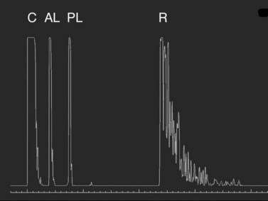
In the contact (applanation) method, the ultrasound probe directly touches the cornea. The contact technique is completely examiner dependent because it requires direct contact and anterior compression of the cornea. See Clip 7.2 Previous studies have demonstrated a mean shortening of AL by 0.1 to 0.33 mm using the contact technique compared with immersion technique.⁷^–¹⁰ In the echogram for the axial eye length measurement, the first spike represents the probe tip placed on the cornea, followed by the anterior lens capsule, posterior lens capsule, vitreous cavity, retina, sclera, and orbital tissue echoes (Figure 7.1). The corneal spike is a double-peaked echo to represent the anterior and posterior surfaces of the cornea. The retinal spike is generated from the anterior surface of the retina. This echo needs to be highly reflective with a sharp 90° take-off from the baseline. The scleral spike is another highly reflective spike just posterior to the retinal spike. The orbital spikes are low reflective spikes behind the scleral spike.

Figure 7.1 Contact A-scan of a normal phakic eye. The spikes correspond to corneal surface (C), anterior (AL) and posterior lens capsule (PL), and retina (R).

Reproduced with permission from: Rocha KM, Krueger RK. Ophthalmic biometry. Ultrasound Clin 2008; 3(2):195–200.¹

Immersion

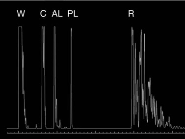
Because the immersion method eliminates compression of the globe, this technique has been shown to be more precise than contact biometry (Figure 7.2). See Clip 7.3 In the immersion technique, a scleral shell filled with fluid is placed over the cornea while the patient lies supine. The most commonly used scleral shells are the Hanson shells (Hansen Ophthalmic Development Laboratory, Coralville, IA, USA) and the Prager shells (ESI Inc., Plymouth, MN, USA). The shells come in different sizes, although the 20 mm shell is the most versatile. The probe is immersed in the fluid overlying the cornea. Clinically, this method is important in eyes with a small AL (high hyperopia, microphthalmos, nanophthalmos). Phakic AL measurement spikes using the immersion technique:

• The initial spike is the tip of the probe, which has no clinical significance. This echo is now moved away from the cornea in immersion and has become visible.

• The other spikes, from left to right on the screen, represent anterior lens capsule, posterior lens capsule, retina, sclera, and the orbital fat.

Figure 7.2 Immersion A-scan of a normal phakic eye. The spikes correspond to waterbath (W), anterior and posterior cornea surface (C), anterior (AL) and posterior lens capsule (PL), and retina (R).

Reproduced with permission from: Rocha KM, Krueger RK. Ophthalmic biometry. Ultrasound Clin 2008; 3(2):195–200.¹

Settings

Most instruments offer the choice of either a manual or automatic (“pattern recognition”) measurement mode. To obtain an AL measurement in manual mode, the examiner determines the A-scan to be measured and depresses a foot pedal to take the measurement. This is the preferred methodology because the examiner can examine the spikes and make sure that they are properly aligned and appropriately gated. In the automatic mode, the machine is programmed to recognize spikes that occur within a preset range from the probe. When the display has a series of spikes which the software recognizes, the instrument will record that measurement. When the automatic mode is in use, the instrument is prone to making errors and giving inadequate measurements. There is also an option of a contact or immersion measurement mode. Make sure this setting is correct, otherwise your measurements will be erroneous. Biometers also have phakic, pseudophakic, and aphakic settings that can be chosen based on the lens status of the patient. Some instruments also have a dense cataract setting. The dense cataract setting is used when the examiner is having difficulty displaying a distinct, high spike from the posterior lens capsule and the retina.¹¹

Velocity settings

Accurate measurements of AL require the use of appropriate sound velocity settings. Sound waves travel at different speeds according to the physical properties of the medium. The ultrasound velocity varies in relation to the medium within the eye and IOL materials (Tables 7.2 and 7.3).^12,¹³ In a normal phakic eye, the average ultrasound velocity is 1555 m s⁻¹. In eyes with a short AL (<20 mm), it is 1560 m s⁻¹, whereas in longer eyes it is 1550 m s⁻¹. This difference is due to an inverse proportional shift in the axial ratio of solid to liquid as the eye increases in length.

Table 7.2 Sound velocities for axial length measurements.

Medium	Velocity (m s⁻¹)
Soft tissue	1550
Cornea	1641
Aqueous / vitreous	1532
Crystalline lens	1641
Silicone oil	980

Reproduced with permission from: Rocha KM, Krueger RK. Ophthalmic biometry. Ultrasound Clin 2008; 3(2):195–200.

Table 7.3 Average sound velocities according to lens status.

Eye types	Velocity (m s⁻¹)
Phakic	1555
Aphakic	1532
Pseudophakic (PMMA)	1556
Pseudophakic (acrylic)	1549
Pseudophakic (silicone)	1476
Phakic (gas)	534
Phakic (silicone oil)	1139
Aphakic (silicone oil)	1052

Reproduced with permission from: Rocha KM, Krueger RK. Ophthalmic biometry. Ultrasound Clin 2008; 3(2):195–200.

The electronic gates

Electronic gates allow ultrasound units to provide an electronic read-out of the AL in millimeters. Biometers are equipped with two or four gates. The two main gates are the “corneal gate” placed in the region of the corneal spike and the “retinal gate” placed in the region of the retinal spike. Instruments equipped with four gates allow positioning of these gates over the leading edges of the echoes generated from the anterior surface of the cornea, the posterior surface of the cornea, the anterior surface of the lens, the posterior surface of the lens, and the anterior surface of the retina.¹⁴ These gates need to be properly monitored and adjusted during AL measurement because certain clinical situations can interrupt normal gating (i.e., dense cataracts, IOLs, etc.). Improper placement of gates can read the measurement between two unrelated surfaces instead of between the cornea and the retina.

Troubleshooting

Errors in an AL measurement are due to improper technique yielding shorter or longer measurements.^15,¹⁶ One of the commonest errors is misalignment of the ultrasound probe with the visual axis or macular surface. When the retinal, lenticular or corneal spikes are of high amplitude and steeply rising without sloping or spikes, the ultrasound beam is most likely on axis. The scleral echo should easily be identified and the orbital fat echoes should descend quickly and at a steep angle. The retinal spike will be present and of high amplitude and can even appear steeply rising, but, if the scleral spike is not as high in amplitude as the retina, the sound beam is misaligned along the nerve. No sclera is present at the optic nerve: If there are no scleral or orbital fat echoes visible, the ultrasound beam is most likely aligned with the optic nerve rather than the macula.¹⁷ See Clip 7.4 Biometry units that are not equipped with an oscilloscope or a screen that displays the actual scan have a high error rate and are definitely not recommended.¹⁴

Comparison of IOL Master® and immersion A-scan

Optimal use

Clinical situations such as a mature or darkly brunescent lens, central posterior subcapsular plaques, corneal scars in the visual axis, and vitreous hemorrhages may interfere with the partially coherent light beams and decrease the signal to noise ratio to the point that may preclude a meaningful measurement. In these cases, immersion A-scan may be the best biometric technique. On the other hand, very difficult immersion ultrasonography measurements, such as eyes with posterior staphylomata or eyes in which the vitreous cavity has been temporarily filled with silicone oil, are more routine with the IOL Master®.⁵

Measuring specific conditions – challenging eyes

Aphakic

The IOL Master® and most ultrasound machines have a setting for aphakic eyes. When setting the measurement mode to aphakic, two gates will be present (on the respective corneal and retinal surfaces), and the biometer will calculate the distance at a velocity of 1532 m s⁻¹, the correct velocity for the aqueous and vitreous.

Pseudophakic

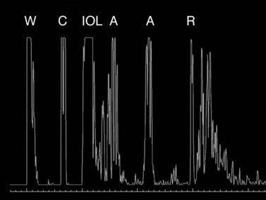
IOLs occasionally need to be exchanged after cataract surgery because of surgical complications or postoperative refractive surprise.¹⁸ Patients who had received older-generation IOLs might request IOL exchange for restoration of more visual function by, for example, correction of presbyopia, astigmatism, glare, etc. Indication for IOL exchange aiming to reduce residual refractive errors increased from 13.9% in the late 1980s to 30–40% in the early 2000s.¹⁸ Ocular biometry in pseudophakic eyes is thus even more important than previously expected.⁶ During the measurement of pseudophakic eyes, the first spike represents the lens implant, followed by multiple signals. IOL implantation causes multiple echoes within the vitreous cavity (Figure 7.3). The first spike (IOL echo) should also be aligned along the visual axis and should be of maximum height. Adjustments should be made according to the ultrasonic velocity of the IOL material. Nevertheless, the identification of retinal spikes can be difficult in some cases because of the proximity of the multiple echoes to the retina spike. In these cases, the examiner should decrease the gain for better identification of the retina spike. Holladay and Prager described a conversion factor to improve the accuracy of the AL measurements in pseudophakic eyes.¹⁹ They considered the implant composition, the center thickness, and the amount of vitreous and aqueous crossed by the ultrasonic beam. The conversion factor was obtained by multiplying the center thickness of the IOL by a factor related to the implant’s ultrasonic velocity.

Figure 7.3 Immersion A-scan of a pseudophakic eye. The spikes correspond to waterbath (W), anterior and posterior cornea surface (C), intraocular lens implant (IOL), and retina (R). Multiple spikes (A; artifacts) are a result of intraocular lens implant.

Reproduced with permission from: Rocha KM, Krueger RK. Ophthalmic biometry. Ultrasound Clin 2008; 3(2):195–200.¹

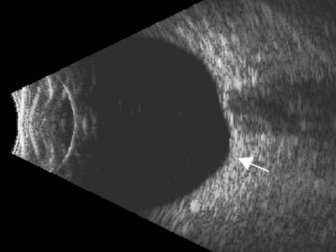
Posterior staphyloma

The possibility of a posterior staphyloma should be considered in all eyes with high axial myopia, particularly when AL is difficult to measure and is greater than 26 mm (Figure 7.4). In these cases, the retinal peak is difficult to capture during the A-scan measurement because the macula may lie on a slope. B-scan is used to confirm the unusual shape of the posterior ocular wall. A combined B/A-scan vector immersion technique is a complementary method that should be considered in these cases.²¹ The combined B/A-scan vector is able to obtain an echogram that highlights the central echoes of the cornea, the anterior and posterior lens, and macula while displaying the optic nerve image. The B-scan is used to adjust the center of the cornea, lens, and fovea.

Figure 7.4 Immersion B-scan at 10 MHz demonstrating posterior pole staphyloma.

Reproduced with permission from: Rocha KM, Krueger RK. Ophthalmic biometry. Ultrasound Clin 2008; 3(2):195–200.¹

Coloboma

Occasionally a retinal coloboma can be undetected if associated with a mature cataract in an eye with unilateral axial myopia.²² As with staphyloma or any other irregularities in the contour of the posterior ocular wall, a retinal coloboma can also cause A-scan readings to be falsely long. The combined B/A-scan technique described above for posterior staphyloma can be employed in patients with coloboma.

Specific guidelines to avoid AL measurement errors

Patient history

Prior to the examination the biometrist and practitioner should ascertain the patient’s history, including any previous ocular surgery or intraocular abnormalities. If for example, the eye is pseudophakic or contains silicone oil, particular sound velocities and examination techniques are necessary in order to obtain reliable measurements. A history of uncontrolled diabetes might increase the possibility of macular thickening. Also, a history of retinal detachment status post scleral buckle placement may explain an increase in AL when compared to the fellow eye.¹¹

Preoperative refraction

One must also keep in mind that AL measurements should match a patient’s precataract refractive error. Hyperopes usually have short eyes whereas myopes usually have long eyes.¹¹

Confirm all asymmetrical measurements

Several scans should be done on each eye. The measurements should cluster around a variance of no more than 0.2 mm. Assuming that the patient is not monocular, both eyes should also be measured. The difference between eyes should be no larger than 0.3 mm unless there is a refractive or known anatomical explanation.²³

Normative data for anterior segment structures

The distribution of AL and other ocular biometric parameters, for example, the corneal radius of curvature or corneal power (K1), anterior chamber depth (ACD), and lens thickness, follow a common Gaussian curve. Multiple investigators have measured AL to establish normal values. In 1980, Hoffer used an immersion technique to examine 7500 eyes and found a mean AL of 23.65 mm (±1.35 mm).²⁴ In 1993, Hoffer repeated these measurements on 450 eyes and obtained a mean AL of 23.56 mm (±1.24 mm). Standard values have also been determined for corneal thickness, anterior chamber depth and thickness of the crystalline lens. The established value for average corneal thickness is 0.55 mm.²⁵ Using an immersion technique, Hoffer has determined that the mean anterior chamber depth in phakic eyes is 3.24 mm (±0.44 mm)²⁴ and the mean thickness of the cataractous lens is 4.63 mm (±0.68 mm).²⁵

Intraocular lens power calculations

First-generation formula

First-generation formulas included regression analysis of previous IOL implantation cases and the predicted IOL position (ACD), which depended upon a specific constant for each IOL. In 1967, Fedorov and colleagues published the first formula for IOL calculation based on schematic eyes.²⁶ Subsequently, Colenbrander²⁷ described his formula, followed by Hoffer in 1974.²⁸ In 1975, Binkhorst published a formula that was widely used in the United States.²⁹ Regression analysis was described by Sanders and Kraff³⁰ in 1980, followed by the SRK-I comparison to the other formulas.³¹ The SRK formula was superior to the other formulas by having a smaller range of error.

Second-generation formula

The predictive relationship between the IOL position within the posterior chamber and the axial length was described to improve the accuracy of first-generation formulas. This direct relationship was calculated by different methods as demonstrated by the SRK-II formula.³²

Third-generation formula

The third-generation formulas assumed that the IOL position was related to the axial length. Long eyes would have a deep anterior chamber, whereas short eyes would have a shallow anterior chamber. It has since become well known that this assumption is not valid; hence, at the extremes of axial length, the third-generation formulas produce considerably variable results.

In 1988, Holladay and colleagues incorporated the surgeon factor (SF) to the second-generation formulas.³³ With this factor, they described the relationship between corneal steepness and the IOL position. The Holladay 1 formula considered the distance from the cornea to the iris plane and from the iris to the posterior chamber IOL position (SF). Retzlaff and colleagues in 1990 modified the Holladay 1 formula by incorporating the A-constants to the SRK/T formula (theoretic).³⁴

Hoffer modified his own formula in 1993 by replacing the regression formula with a theoretic formula (Hoffer Q).³⁵ The Hoffer Q formula has been demonstrated to be clinically more accurate than the Holladay 1 and SRK/T formulas in eyes shorter than 22.0 mm.

Fourth-generation formula

The fourth-generation formulas introduced innovative approaches for IOL calculation as follows.

The Haigis formula represents a significant improvement over other two-variable formulas. It uses three IOL and surgeon-specific constants (a₀, a₁ and a₂) with more effective lens position settings using the following formula:³⁶

The A-constant mainly moves the prediction curve up or down very similar to A-constant, Surgeon Factor (SF) and ACD respectively in SRK/T, Holladay 1 and Hoffer-Q. The constant a₁ is linked to the ACD (distance of the corneal vertex to the anterior lens capsule), which can alter and more accurately determine the position and the shape of the IOL power prediction curve. It also includes the constant a₂, which is linked to the AL (distance from the corneal vertex to the macula). The constants are derived by regression analysis and produce an IOL-specific and surgeon-specific factor for different anterior chamber depths and axial lengths. Corneal power measurements are not required in the calculation of the effective lens position (ELP); thus, errors in measurement of the anterior corneal radius and the prediction of post-operative ELP are avoided. The main limitation of the Haigis formula is that the three constants must be derived by regression analysis based on surgeon-specific data of a large number of cases (n > 200) containing a wide range of axial lengths.³⁷ If the constants are not optimized, the accuracy of the Haigis formula is similar to the Hoffer-Q.

The Holladay 2 formula was introduced in 1998 and is one of the most precise theoretical formulas available. The input of several variables is needed: IOL thickness, corneal power, corneal diameter, ACD measurements, lens thickness, axial length, refractive error, and age to obtain and refine the estimated scaling factor (ESF). A database of 35 000 patients was used to create the Holladay 2 formula. It has an excellent precision in all axial lengths. The lens thickness is one of the variables and must be measured by the A-scan or by the Lenstar system. The current version of the IOL Master® does not calculate the lens thickness.

Selection of the best formula

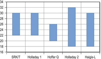
In 1993 Hoffer published an important article regarding the eye’s axial length and formulas. It had been shown that, within the normal range of axial length (22.0–24.5 mm) and central corneal powers ranging from 41.00D to 46.00D, almost any modern IOL power calculation formula yields the same or similar and accurate results; however, at the extremes of axial length, the formulas begin to differ.³⁵ The Holladay 1 formula was the most accurate in eyes from 24.5 to 26.0 mm, whereas the SRK/T worked more adequately in very long eyes (>26.0 mm). The Hoffer Q formula was the most accurate for short eyes (<22.0 mm). More recently, the performance of the Holladay 2 formula was shown to be comparable with that of the Hoffer Q formula in short eyes (<22.0 mm) in a study with 317 eyes.³⁸ Nevertheless, the original Holladay 1 formula was more accurate in eyes with average and medium–long axial lengths. The great advantage of the fourth-generation formulas, such as Holladay 2 or Haigis (with the optimized constants) is the excellent results in a much greater range of axial lengths (Figure 7.5).

Figure 7.5 Expected error of less than 0.50D in IOL calculations with 3rd and 4th generation formulas in different axial lengths.

Post-refractive surgery

Laser in situ keratomileusis (LASIK), photorefractive keratectomy (PRK), and radial keratotomy (RK) change the corneal architecture by flattening the cornea surface. This represents a great challenge for a precise IOL calculation. LASIK and PRK mainly change the anterior curvature of the cornea, while RK for myopia correction flattens both the anterior and posterior cornea curvatures. As a result, RK surgery is less susceptible to error compared to laser vision correction. Three errors commonly occur when calculating an IOL for these patients:

The measurement of the anterior corneal radius in topography or keratometry is systematically incorrect, since it is not performed on the central cornea (flatter in myopic corrections), but more peripherally. Keratometry readings in flatter corneas can also represent data further in the periphery compared to normal cornea (usually the 3 mm zone). After myopic laser surgery, the measured radius of curvature will be too small (overestimate the corneal power in diopters).

A second independent error results from the commonly applied assumption of corneal power from the anterior radius in topography or keratometry measurements. A constant ratio of anterior to posterior radius (e.g., Gullstrand-ratio: 7.7/6.8) is implicitly assumed. This ratio, however, has been changed by the refractive procedure (especially with laser vision correction). After excimer ablation for myopia, both errors will lead to an overestimation of the power of the cornea thus causing an underestimation of the necessary IOL power. The opposite happens when dealing with hyperopic correction where the errors will lead to an overestimation of the IOL power.

The commonly used 3^rd generation formulas (SRK/T, Holladay 1 and Hoffer-Q) have a prediction algorithm for the postoperative effective lens position that derives directly from the corneal power. The formula assumes that steeper corneas are related to longer eyes with a posterior ELP, while flat corneas are related to small eyes, with reduced anterior chamber depth and anterior displaced ELP. The problem is that the formulas use flat K values found in after a myopic laser ablation to assume the eye is short, with an anterior displacement of the ELP. This error also underestimates the IOL power.

As seen above, the three main errors for IOL calculation after myopic treatments lead to an underestimation of IOL power and consequently a postoperative hyperopic surprise. Several methods are described to estimate the real post-refractive surgery K value and to include in formula the actual effective lens position. Despite the common sense that the clinical history method is the gold standard to calculate the corneal power in corneas that have undergone refractive surgery, the difficulty to obtain reliable preoperative data can induce large errors in IOL calculation. Recent studies have shown less variability and better results in methods that estimate corneal power based on change of the spherical equivalent than in methods that use pre-refractive surgery readings.³⁹

Double K formula method

A very common source of postoperative error following refractive surgery is related to the ELP calculation. The ELP is the distance between the surfaces of the cornea (vertex) to the plane of the IOL. Third-generation formulas assume the K power and axial length to estimate the ELP. When using these formulas, very flat keratometric corneal power following refractive surgery will produce a falsely shallow postoperative ELP. As a result, the calculated IOL power will be underestimated, ensuing in a hyperopic error.

In 2003 Chamon described a “double K” method by using the preoperative and postoperative corneal power for IOL calculation after refractive surgery using the Holladay 1 formula.⁴⁰ The preoperative K value was determined by topography and the postoperative K value by the clinical history method. When the preoperative K value is unknown, 44.0D is considered as the preoperative value and the effective refractive power (EffRP) of the Holladay Diagnostic Summary–EyeSys Corneal Analysis System (Dallas, Texas) as the postoperative value.

Aramberri published the double K method using the SRK/T formula.⁴¹ The SRK/T formula was modified to use the preoperative K value to estimate the ELP and the post-refractive surgery K value (clinical history method) to calculate IOL power by the vergence formula. The Holladay 2 formula contains the double K entry for post-refractive surgery cases. If the preoperative K value is unknown, the formula suggests the 43.86D value.

Clinical history method

The clinical history method was the first to be described and is the easiest to understand. However, it relies on accurate preoperative data, which sometimes can be unavailable or unreliable. This is the main reason for getting accurate measurements before proceeding to refractive surgery. Both the preoperative corneal power (keratometry) and the preoperative and postoperative refractive errors are necessary to acquire the final K value using this method. Inaccurate preoperative data and a change in postoperative refraction caused by changes in the lens (and not in the cornea) can lead to undesirable outcomes.

The estimate of the central corneal power after refractive surgery is obtained by subtracting the difference between preoperative and postoperative spherical equivalent error from the average keratometry power before refractive surgery. The spherical equivalent pre and postoperative must be vertex distance corrected (corneal plane). The following formula should be used:

K_pre = average keratometry power before refractive surgery

SE_pre = spherical equivalent before refractive surgery

SE_aft = spherical equivalent after refractive surgery.

Example

K_pre = 44.50D

SE_pre = −5.00 (−4.72 after vertex distance correction)

SE_post = −0.25D

Feiz–Mannis method

The method described by Feiz and Mannis is empiric and needs accurate pre-refractive surgery data.⁴² It consists of of calculating the IOL power with the values before refractive surgery and then adding the change in refraction divided by 0.7.

ΔD = stable change in refraction (spherical equivalent) after refractive surgery at the spectacle plane. The value is negative in myopic treatments, which will lead to higher IOL power.

Example

IOL power calculated with preop data = +10.2D

Change in spherical equivalent after refractive surgery = −5.5D

The ELP is calculated using the preoperative data and thus, no adjustments are needed to this method. This technique is the least likely formula to result in hyperopic surprise after cataract surgery and can be used in conjunction with other formulas to indicate an upper limit of IOL power. It should be noted that this formula may overestimate the IOL power and result in myopic surprise.

Wang–Koch–Maloney method

This method, a modification of the previous method described by Maloney, does not require any preoperative data to calculate the K value. This method needs to be used in conjunction with a double K formula or the Holladay 2 to ensure proper ELP and has shown good results with very low variability compared to the clinical history method.^39,⁴³ The formula is based on the principle that refractive surgery changes the normally fixed relation between the anterior and posterior cornea curvature, and regular topography maps use a fudged index to estimate the corneal power based on the anterior curvature. The idea is to regress this calculation to find the power of the anterior curvature and then subtract the value of the posterior curvature (which remains unchanged in laser vision correction).

The K value is found by positioning the cursor on the exact center of the axial map in the Zeiss Atlas topography, multiply by 1.114 to find the value of the central anterior curvature and then subtract the average power of the posterior curvature (it is a minus lens) according to the following formula:

Example

Topographic central cornea adjustment method

This method uses the magnitude of change in the spherical equivalent in the spectacle plane after surgery to estimate the induced change in the relation between the anterior and posterior curvature. Then you correct the formula used by the topographer to estimate the corneal power based on the anterior curvature.⁴³ The central corneal power value to be used in this method can be the average of the power in 1, 2, 3, and 4 mm zones in the Zeiss Atlas topographer or the effective refractive power found in the EyeSys topographer. One of the disadvantages is that this method cannot be used with other topography systems.

The formula used is the following:

Example

Masket method and modified Masket method

A linear relationship observed in a large database of patients of the amount of laser vision correction spherical equivalent and the induced error in topography was used to create an empiric regression formula to correct the K value obtained by topography.⁴⁴ This is called the Masket method. The IOL should be calculated using the simulated keratometry and Holladay 1 formula for eyes longer than 23.00 mm or Hoffer-Q for eyes under 23.00 mm. The double-K method should not be used. The IOL power should then be corrected by the following factor (increase the IOL power in myopic corrections and decrease in hyperopic):

Example

IOL calculated with simulated keratometry: +17.00

Change in spherical equivalent: −4.00

Another analysis of a different dataset found better results with different values to correct the K value. The structure of the method is the same; it is called the modified Masket method and is represented by the following formula:

The methods can be used after myopia and hyperopia corrections. The disadvantage is that knowledge of the amount of prior laser vision correction is necessary.

Corneal bypass method

In this technique, the need for dealing with corneal power measurements in a post-refractive surgery cornea is avoided. However, the pre-refractive surgery keratometry values are required and used together with the postoperative axial length in a regular Holladay 1 formula without further modifications. In contrast, instead of aiming for plano, the target should be the pre-refractive vision spherical equivalent subtracted by the post-refractive vision correction spherical equivalent.⁴⁵

Example

Pre-excimer spherical equivalent: −5.00D

Post-excimer spherical equivalent: +0.50D

Target for IOL calculation: −5.00 − (+0.50)

Target for IOL calculation: −5.50

One of the most important limitations regarding this method, besides the need for precise pre-excimer data, is that we must have an accurate and stable postoperative refraction. This can be altered by the cataract, which can decrease the accuracy of the method. Another option is target for the amount of myopia treated, which can lead to errors if the intended amount of myopia treated was different than the amount achieved.

Shammas method

Another option when the preoperative data is not available is to use the Shammas method.⁴⁶ It is very similar in theory to the Wang–Koch–Maloney method. Using regression analysis, this method estimates the post-refractive corneal power by adjusting the measured post-refractive corneal readings (K_post): K = 1.14 × K_post – 6.8.

In this formula, the preferred data to be used as a postoperative keratometry is the average of 1 mm, 2 mm, and 3 mm annular powers on the Numerical View from the Zeiss Humphrey Atlas topographer. The IOL Master® Ks can be used if the Atlas topographic data are not available.

Contact lens method

The hard contact lens method requires a known contact lens base curve (BC) and refractive power (PC) in diopters, and the spherical equivalent refraction with (SE_cl) and without (SE) the contact lens. The great advantage of this method is not requiring preoperative data. By this method, the final estimate corneal power (K) after refractive surgery is calculated as follows:

Ideally, a PMMA contact lens is preferred compared to RGP. The final estimated corneal power should then be used in a double K or fourth-generation formula to ensure the proper ELP. The contact lens method should not be used when a cataract or other media opacities compromise the accuracy of the refraction.⁴⁷

Haigis-L

The corneal power in the Haigis-L formula is calculated based on a corrected corneal radius measured by the IOL Master® keratometry. The corneal radius is corrected by a specific algorithm, one for post-myopia correction, and another for posthyperopia correction. The corrected radius is then transformed to diopters and the result used in the regular Haigis formula to calculate the IOL power. The great advantage of this technique is to calculate the correction factor in corneal radius, which is not influenced by the problems found in calculating power based on curvature in a post-refractive surgery cornea. The ELP is not a problem, since this formula does not use corneal power in its calculations for the IOL position.

This is the algorithm to correct the corneal radius in a postmyopic ablation:

Pentacam®

There are two main sources of error in using a topographer to estimate the real central corneal power. The first is that there is a change in relationship between the anterior and posterior curvatures. Since the topographer measures only the anterior curvature and uses a fudged index based on a fixed relationship to estimate the corneal power, the measurements are inaccurate when this relationship is changed (e.g., eyes with previous refractive surgery). The second is that a camera is located at the center of the topographer, thus the very central value cannot be measured. The Pentacam® utilizes a scheimpflug camera which rotates 360° about the eye taking multiple scans of the eye resulting in a three-dimensional image of the cornea and anterior segment of the eye. This scheimpflug technology is able to measure the posterior surface and then estimate the real power. It is also capable of measuring the very central K. Two indices can be used with Pentacam® in eyes that had previous refractive surgery: the central K and the equivalent K-reading (EKR). The EKR is a value measured by scheimpflug similar to the standard keratometry or topography on the front surface, adjusted for the effect of the back surface power difference from normal.⁴⁸ The recent literature shows some conflict in the results with the use of the EKR, with some variability and hyperopic surprises being reported.⁴⁹ The main problem seems to be low accuracy of keratometry readings in scheimpflug images of the anterior curvature compared to placido-based technology.

Galilei®

The Galilei® is a placido-based topographer integrated with a dual-scheimpflug system. It can deliver information about the anterior surface in a placido-based system (similar to a regular topographer and more accurate than scheimpflug technology) and the posterior surface can be mapped through the scheimpflug system. The idea is to use this device to measure the real central corneal power in post-refractive surgery eyes because it can measure both anterior and posterior corneal surfaces, instead of measuring only the anterior surface and trying to estimate the power of the posterior surface (as happens in regular topographers). The accuracy and reproducibility seems to be greater compared to the Pentacam®, which is a single scheimpflug system.

The index to be used in eyes that had previous refractive surgery is the total corneal power. It is composed of ray tracing data over the central 4 mm zone of corneal thickness, anterior and posterior curvatures. This data can be used in a double-K formula or be entered in the ASCRS IOL calculator website. The first results show a low standard deviation and low average error with almost no hyperopic surprises (the majority of the results were within −0.50D of myopia).⁵⁰

Consensus K technique

To avoid errors with a specific method to calculate the real K value in corneas after refractive surgery, it is suggested to use the consensus K technique, in which several different methods are used. The results show that outcomes with this technique are better than relying on any individual method.⁵¹ The method includes calculating IOL power by all available formulas; eliminate the highest and lowest values (outliers). The average of the remaining should be calculated (ideally all the values should be within 0.75D).

IOL calculation after hyperopic treatments

Hyperopic treatments are not as challenging to acquire an accurate corneal power as myopic treatments. The major reason is that the ablation occurs outside the central cornea. The main error encountered after hyperopic ablations is an underestimation of the corneal power (resulting in a myopic surprise) compared to the overestimation in the myopic treatments (hyperopic surprise). Usually a smaller central zone corneal power in the topography map is sufficient for an accurate value. Some authors recommend the average of the 1 mm, 2 mm and 3 mm annular power rings of the numerical view of the Zeiss Humphrey Atlas topographer.⁵² The effective refractive power (EffRP) of the EyeSys topographer can also lead to good results. After a higher hyperopic treatment (over 3D) a small correction in the corneal power must be made to avoid the myopic surprise. A double-K formula or Holladay 2 should be used to ensure proper ELP. The Haigis-L formula for hyperopic treatments can also be used with very good results.

Post-radial keratotomy and cataract surgery

Special attention should be given to patients with previous RK who undergo cataract surgery. Transient hyperopia is commonly observed in the immediate postoperative period.^53,⁵⁴ The stromal edema around the radial incisions and even the opening of the incisions flatten the center of the cornea. The hyperopic shift may need an average of 8 to 12 weeks to completely resolve. Any hasty decision, such as IOL exchange or laser corrections, should not be taken during this period.