CHAPTER 17 Magnetic Resonance Evaluation of Blood Flow
DESCRIPTION OF TECHNICAL REQUIREMENTS
Phase Contrast Magnetic Resonance Imaging
Velocity-encoded cine phase contrast MRI employs a bipolar gradient pulse to encode the velocity of moving protons. The two lobes of the bipolar gradient pulse are equal in strength but opposite in orientation, one positive, the other negative. A stationary proton will experience equal and opposite gradients that cancel one another and will have no resulting phase shift. However, a moving proton will not experience an equal but opposite second lobe of the gradient pulse and consequently will acquire a phase shift (Fig. 17-1). The angle of acquired phase shift is proportional to the velocity of the moving proton. An MRI sequence with this type of bipolar gradient is thus flow sensitive.
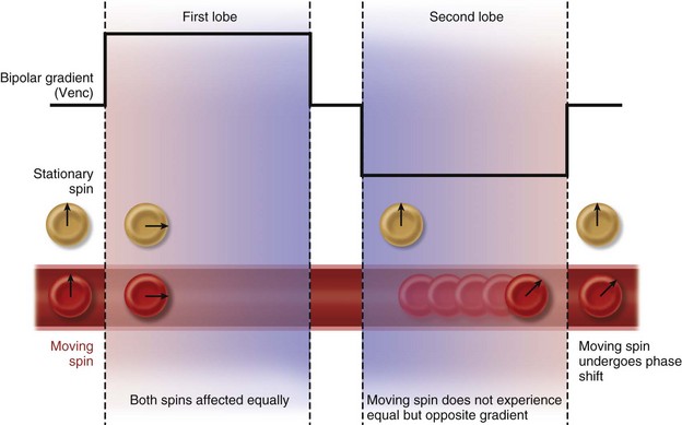
 FIGURE 17-1 Diagram of the effect of bipolar gradients on stationary and moving spins. Venc, velocity encoding value.
(Modified from Westbrook C, Roth CK, Talbot J. MRI in Practice, 3rd ed. Oxford, Wiley-Blackwell, 2005.)
Flow-Encoding Axes
Flow quantification is performed by prescribing an imaging plane orthogonal to the direction of flow within a vessel. During postprocessing, the borders of the vessel are delineated with a flexible region of interest for each segment of the cardiac cycle. This creates a cross-sectional area for each time point and defines the pixels that contain velocities representing intravascular flow. The spatial mean velocity is then calculated from these pixels and multiplied by the cross-sectional area for each time point in the cardiac cycle (Fig. 17-2). The result is blood flow calculated in milliliters per heartbeat.1
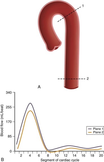
 FIGURE 17-2
Pressure gradients can be estimated with the modified Bernoulli equation, ΔP = 4ν2, where ΔP is the peak pressure gradient in millimeters of mercury and ν is the peak blood flow velocity in meters per second. Unlike flow quantification, phase contrast imaging planes may be prescribed in a parallel or perpendicular orientation with respect to the direction of blood flow to capture the point of peak velocity of flow downstream from a stenosis (Fig. 17-3). It is important to select a relatively high velocity encoding (Venc) value because peak velocities associated with stenotic valves can exceed 5 m/sec.2
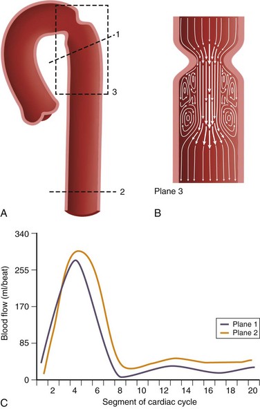
 FIGURE 17-3 A and B, Two-dimensional velocity-encoded cine phase contrast scan planes in the proximal (plane 1) and distal (plane 2) descending thoracic aorta for quantification of collateral blood flow in coarctation of the aorta. Plane 3 is prescribed in the direction of flow to measure peak velocity, which is used to derive the pressure gradient across the stenosis used in the modified Bernoulli equation.11 C, Typical aortic blood flow with two-dimensional velocity-encoded phase contrast MR imaging. Note that the distal blood flow (plane 2) is higher than the proximal flow (plane 1). The area between the curves represents collateral flow.
Velocity Encoding
Phase contrast MRI can be optimized for different velocities of blood flow. The encoding velocity of a given sequence, or Venc, is selected on the basis of the maximum anticipated velocity of the blood flow of interest. The scanner will use this value to adjust the amplitude and duration of the phase contrast bipolar gradients so that a proton moving at the selected Venc value will give rise to a phase shift of 180 degrees. For example, for a Venc value of 100 cm/sec, the range of phase shifts will be adjusted to encode velocities from −100 cm/sec to +100 cm/sec (Fig. 17-4). The lower the Venc value selected, the greater the sensitivity to slower flow but also the stronger the required gradients and the longer the repetition time (TR) of the sequence. An ideal Venc value is slightly greater than the maximum expected velocity.
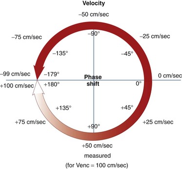
 FIGURE 17-4
Imaging Limitations and Pitfalls
There are some pitfalls to be aware of in employing phase contrast MRI for blood flow quantification. Signal aliasing will occur if the peak velocity of blood flow surpasses the Venc value at any point in the cardiac cycle. This phenomenon takes place because positive velocities that surpass the Venc value will give rise to phase shifts that are interpreted as negative velocities (e.g., a phase shift of 185 degrees will be interpreted as −175 degrees). On phase images, areas of aliasing are easily identifiable: the sudden loss of signal in regions of maximum signal brightness (Figs. 17-5 and 17-6).
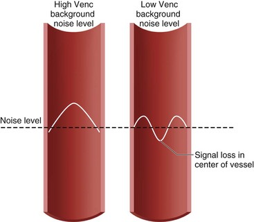
 FIGURE 17-5 Diagram of aliasing with low but not with high velocity encoding value (Venc).
(Modified from Westbrook C, Roth CK, Talbot J. MRI in Practice, 3rd ed. Oxford, Wiley-Blackwell, 2005.)
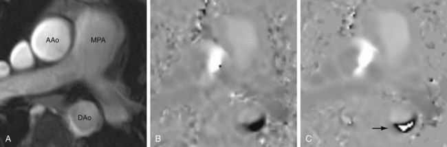
 FIGURE 17-6
Underestimation of velocity and flow can occur if a vessel is not evaluated in a plane orthogonal to the direction of flow or if partial volume averaging occurs. In addition, peak flow velocity downstream of a stenosis, and thus the associated pressure gradient, can be underestimated for two reasons: (1) as the accuracy of peak velocity measurement is dependent on temporal resolution, the value may be underestimated by MRI compared with echocardiography, which has a higher temporal resolution; and (2) the precise, three-dimensional location of the peak velocity downstream from a stenosis may not be included in the two-dimensional phase contrast evaluation.3,4
TECHNIQUES
Technique Description
Valvular Disease
Precise quantification of aortic, pulmonary, and mitral regurgitation has been demonstrated with phase contrast MRI.5–7 Aortic and pulmonary regurgitant volume can be quantified directly, resulting in more accurate and reproducible data than with echocardiography, by which blood flow is estimated on the basis of the apparent size of flow jets, which can be significantly affected by imaging parameters and orientation. The imaging plane is prescribed perpendicular to the direction of blood flow at approximately 1 to 2 cm above the level of the semilunar valve in question (Fig. 17-7). Valvular regurgitant fraction is the ratio of retrograde to antegrade flow across a valve.
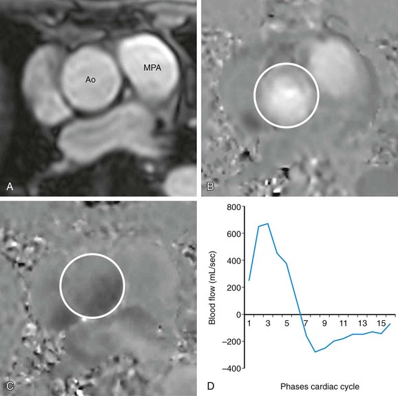
 FIGURE 17-7
Mitral regurgitation can also be assessed directly, but through-plane movement of the valve during systole may introduce significant error.8 Another approach for estimation of mitral regurgitation is subtraction of the flow in the aorta during systole (left ventricular outflow) from flow across the mitral valve during diastole (left ventricular inflow); the base of the heart is less prone to movement during diastole, so by prescribing a two-dimensional plane across the mitral valve during end-diastole, diastolic flow can be reliably calculated. Assuming normal aortic valve function, any difference between the outflow and inflow measurements can be attributed to mitral regurgitation.5 Tricuspid regurgitation can be estimated in a similar fashion from measurements of pulmonic outflow and right ventricular inflow.
The degree of valvular stenosis is estimated by use of the modified Bernoulli equation, ΔP = 4ν2 (discussed earlier in the section on flow-encoding axes), which is also used routinely for Doppler echocardiography. The technique has demonstrated good accuracy compared with Doppler echocardiography for both mitral and aortic stenosis.9,10
Aortic Coarctation
Aortic coarctation is narrowing of the aortic arch that restricts forward flow at or near the junction with the descending aorta. MRI can lend to the evaluation and management of coarctation by providing both anatomic and functional data on the location and degree of stenosis. Specifically, phase contrast MRI allows quantification of the functional significance of coarctation in two ways: (1) estimation of the pressure gradient across the lesion by using the maximum associated flow velocity in conjunction with the modified Bernoulli equation as discussed elsewhere11 and (2) quantification of collateral flow.
Collateral flow arises in coarctation as blood must find an alternate path to the descending thoracic aorta and below. It indicates a hemodynamically significant lesion that may require intervention. Evaluation of collateral flow is achieved by prescribing imaging planes orthogonal to aortic blood flow just distal to the coarctation and at the level of the diaphragm (Figs. 17-3 and 17-8). In healthy individuals, blood flow will decrease by approximately 7% over this interval spanning the descending aorta.12 In hemodynamically significant coarctation, however, blood flow will increase rather than decrease over this interval as blood bypassing the coarctation will be delivered to the distal descending aorta through collaterals; the percentage increase in blood flow gives a quantitative measure of the degree of collateralization.12–14 Study of surgically created coarctation in a porcine model confirms that phase contrast MRI is an accurate method of measuring collateral flow and that these collaterals develop within weeks.15
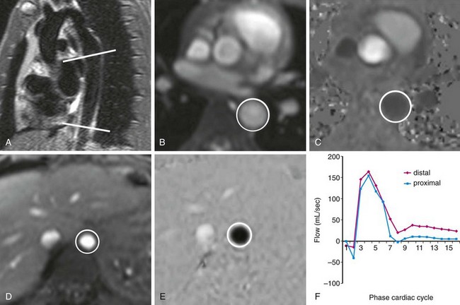
 FIGURE 17-8
Shunts
Quantification of shunt severity is performed clinically to determine if a patient may need surgery or to assess postsurgical outcomes. Intracardiac shunt quantification is achieved with phase contrast MRI by determining the ratio of flow in the pulmonary artery to that in the aorta, referred to as the Qp:Qs ratio, where Qp is the net flow in the main pulmonary artery and Qs is the net flow in the ascending aorta. This type of analysis can be used for both left-to-right and right-to-left shunts; the shunted volume is the difference between the pulmonary and aortic blood flow in either case. Phase contrast MRI has been deemed a first-line clinical study for quantification of shunt volume.16
Measurement of the Qp:Qs ratio is performed with two separate phase contrast acquisitions orthogonal to the direction of blood flow in the main pulmonary artery and ascending aorta, both at approximately 1 cm above the respective semilunar valves (Fig. 17-9). As the placement of this plane will be distal to the coronary ostia in the aorta, aortic flow will be approximately 3% to 5% less than pulmonic flow because of coronary runoff. A normal Qp:Qs ratio, therefore, should be slightly greater than 1. MRI-based measurement of Qp : Qs ratio in this fashion has been extensively validated.17–20
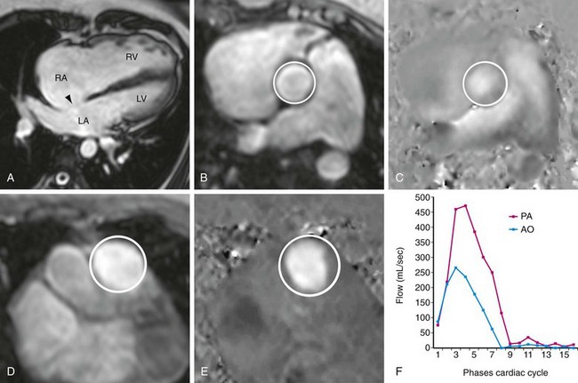
 FIGURE 17-9
Pulmonary Flow Evaluation
Phase contrast MRI can be used to assess differential flow in the right and left pulmonary arteries and relative flow within the pulmonary veins. Branch pulmonary artery stenosis, which can be seen after arterial switch repair performed for transposition of the great vessels, may go undetected with other imaging modalities.21 Direct quantification of blood flow to both lungs is crucial for determination of the hemodynamic significance of such a stenosis. Measurement of differential pulmonary flow is achieved with two phase contrast acquisitions orthogonal to the direction of blood flow in the proximal right and left pulmonary arteries (Fig. 17-10). The normal blood flow distribution is 55% to the right lung and 45% to the left lung.
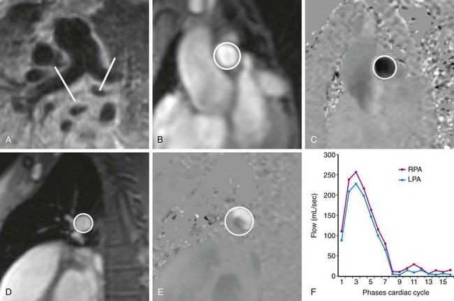
 FIGURE 17-10
MR blood flow evaluation has also been used clinically to assess pulmonary venous obstruction22 and to characterize the complex postsurgical pulmonary inflow in patients after total cavopulmonary connection, with quantification of the relative contributions of the superior and inferior caval veins to the right and left lungs.23 In addition, some investigators have proposed use of the time-resolved velocity data that underlie MR flow evaluations to noninvasively estimate the degree of pulmonary artery hypertension.24
Time-Resolved, Three-Dimensional Phase Contrast MRI
Acquisition of three-dimensional phase contrast data in a time-resolved fashion over the cardiac cycle for an imaging volume that contains the heart and great vessels is an attractive approach to cardiac MRI flow evaluation, but one that has been limited in its clinical application by long scan time. Work in the early 1990s with two-dimensional planes stacked to achieve three-dimensional data sets showed the utility of this type of imaging for uncovering of complex, secondary aortic blood flow characteristics such as helices and vortices, which are not easily appreciated by two-dimensional imaging.25 More recently, true three-dimensional phase contrast acquisitions have been validated, and time-saving measures such as parallel imaging and other approaches to k-space subsampling have been implemented to make this type of comprehensive MR flow evaluation a more viable clinical tool.26–28 The technique has been termed flow-sensitive four-dimensional MRI or simply four-dimensional flow, where the fourth dimension refers to time, and seven-dimensional flow, referring to the seven data components that are encoded for each voxel that composes a data set.
Advantages of this technique include complete temporal and spatial coverage of the vascular area of interest, continuous breathing, no requirement for prospective placement of two-dimensional planes for phase contrast acquisition, and a variety of unique visualization and quantification options for velocity data that are not available by conventional two-dimensional phase contrast imaging. Rich and extensive data analysis is possible in the postprocessing stage with appropriate software. Interactive navigation throughout these volumetric data sets allows evaluation of blood velocity and flow in user-defined regions of interest at any phase of the cardiac cycle (Fig. 17-11). Three-dimensional visualization tools such as streamlines and particle traces allow four-dimensional visual presentation of secondary blood flow features that may not otherwise be evident (Figs. 17-12 and 17-13).
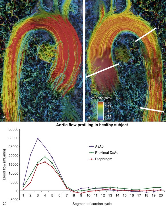
 FIGURE 17-11
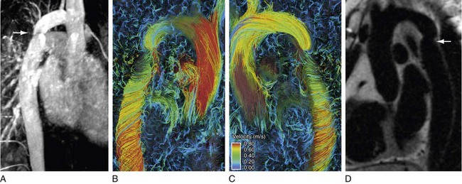
 FIGURE 17-12
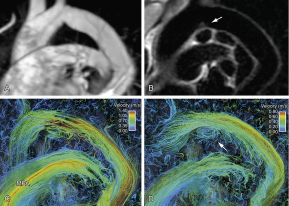
 FIGURE 17-13
Secondary Parameters
Wall shear stress refers to the force per unit area exerted on the vascular wall by fluid in motion in a tangential plane. Abnormal shear values have been strongly implicated in atherogenesis.29 Recently, this parameter has been estimated by use of near wall velocity gradients generated by three-dimensional phase contrast MRI and reported for the carotid arteries as well as for thoracic and intracranial aneurysms.30–33 Confirmation of these reported shear stress values with an accepted standard such as computational fluid dynamics is forthcoming.
Relative pressure mapping has been demonstrated and validated in vivo by use of multidirectional velocity data and the Navier-Stokes equations.34,35 Pulse wave velocity, which reflects the degree of vascular stiffness, is another secondary parameter that can be estimated with time-resolved velocity data, although a much higher temporal resolution than that typically provided by the three-dimensional phase contrast sequence is required for accurate calculation.36


Glockner JF, Johnston DL, McGee KP. Evaluation of cardiac valvular disease with MR imaging: qualitative and quantitative techniques. Radiographics. 2003;23:e9.
Higgins CB, Sakuma H. Heart disease: functional evaluation with MR imaging. Radiology. 1996;199:307-315.
Malek AM, Alper SL, Izumo S. Hemodynamic shear stress and its role in atherosclerosis. JAMA. 1999;282:2035-2042.
Markl M, Chan FP, Alley MT, et al. Time-resolved three-dimensional phase-contrast MRI. J Magn Reson Imaging. 2003;17:499-506.
Pennell DJ, Sechtem UP, Higgins CB, et al. Clinical indications for cardiovascular magnetic resonance (CMR): Consensus Panel report. Eur Heart J. 2004;25:1940-1965.
Varaprasathan GA, Araoz PA, Higgins CB, Reddy GP. Quantification of flow dynamics in congenital heart disease: applications of velocity-encoded cine MR imaging. Radiographics. 2002;22:895-905.
1 Varaprasathan GA, Araoz PA, Higgins CB, Reddy GP. Quantification of flow dynamics in congenital heart disease: applications of velocity-encoded cine MR imaging. Radiographics. 2002;22:895-905.
2 Glockner JF, Johnston DL, McGee KP. Evaluation of cardiac valvular disease with MR imaging: qualitative and quantitative techniques. Radiographics. 2003;23:e9.
3 Higgins CB, Sakuma H. Heart disease: functional evaluation with MR imaging. Radiology. 1996;199:307-315.
4 Tang C, Blatter DD, Parker DL. Accuracy of phase-contrast flow measurements in the presence of partial-volume effects. J Magn Reson Imaging. 1993;3:377-385.
5 Dulce MC, Mostbeck GH, O’Sullivan M, et al. Severity of aortic regurgitation: interstudy reproducibility of measurements with velocity-encoded cine MR imaging. Radiology. 1992;185:235-240.
6 Rebergen SA, Chin JG, Ottenkamp J, et al. Pulmonary regurgitation in the late postoperative follow-up of tetralogy of Fallot. Volumetric quantitation by nuclear magnetic resonance velocity mapping. Circulation. 1993;88:2257-2266.
7 Fujita N, Chazouilleres AF, Hartiala JJ, et al. Quantification of mitral regurgitation by velocity-encoded cine nuclear magnetic resonance imaging. J Am Coll Cardiol. 1994;23:951-958.
8 Hundley WG, Li HF, Willard JE, et al. Magnetic resonance imaging assessment of the severity of mitral regurgitation. Comparison with invasive techniques. Circulation. 1995;92:1151-1158.
9 Kilner PJ, Manzara CC, Mohiaddin RH, et al. Magnetic resonance jet velocity mapping in mitral and aortic valve stenosis. Circulation. 1993;87:1239-1248.
10 Heidenreich PA, Steffens J, Fujita N, et al. Evaluation of mitral stenosis with velocity-encoded cine-magnetic resonance imaging. Am J Cardiol. 1995;75:365-369.
11 Kilner PJ, Firmin DN, Rees RS, et al. Valve and great vessel stenosis: assessment with MR jet velocity mapping. Radiology. 1991;178:229-235.
12 Steffens JC, Bourne MW, Sakuma H, et al. Quantification of collateral blood flow in coarctation of the aorta by velocity encoded cine magnetic resonance imaging. Circulation. 1994;90:937-943.
13 Holmqvist C, Ståhlberg F, Hanséus K, et al. Collateral flow in coarctation of the aorta with magnetic resonance velocity mapping: correlation to morphological imaging of collateral vessels. J Magn Reson Imaging. 2002;15:39-46.
14 Araoz PA, Reddy GP, Tarnoff H, et al. MR findings of collateral circulation are more accurate measures of hemodynamic significance than arm-leg blood pressure gradient after repair of coarctation of the aorta. J Magn Reson Imaging. 2003;17:177-183.
15 Chernoff DM, Derugin N, Rajasinghe HA, et al. Measurement of collateral blood flow in a porcine model of aortic coarctation by velocity-encoded cine MRI. J Magn Reson Imaging. 1997;7:557-563.
16 Pennell DJ, Sechtem UP, Higgins CB, et al. Clinical indications for cardiovascular magnetic resonance (CMR): Consensus Panel report. Eur Heart J. 2004;25:1940-1965.
17 Arheden H, Holmqvist C, Thilen U, et al. Left-to-right cardiac shunts: comparison of measurements obtained with MR velocity mapping and with radionuclide angiography. Radiology. 1999;211:453-458.
18 Powell AJ, Maier SE, Chung T, Geva T. Phase-velocity cine magnetic resonance imaging measurement of pulsatile blood flow in children and young adults: in vitro and in vivo validation. Pediatr Cardiol. 2000;21:104-110.
19 Sieverding L, Jung WI, Klose U, Apitz J. Noninvasive blood flow measurement and quantification of shunt volume by cine magnetic resonance in congenital heart disease. Preliminary results. Pediatr Radiol. 1992;22:48-54.
20 Brenner LD, Caputo GR, Mostbeck G, et al. Quantification of left to right atrial shunts with velocity-encoded cine nuclear magnetic resonance imaging. J Am Coll Cardiol. 1992;20:1246-1250.
21 Gutberlet M, Boeckel T, Hosten N, et al. Arterial switch procedure for D-transposition of the great arteries: quantitative midterm evaluation of hemodynamic changes with cine MR imaging and phase-shift velocity mapping—initial experience. Radiology. 2000;214:467-475.
22 Videlefsky N, Parks WJ, Oshinski J, et al. Magnetic resonance phase-shift velocity mapping in pediatric patients with pulmonary venous obstruction. J Am Coll Cardiol. 2001;38:262-267.
23 Houlind K, Stenbøg EV, Sørensen KE, et al. Pulmonary and caval flow dynamics after total cavopulmonary connection. Heart. 1999;81:67-72.
24 Laffon E, Vallet C, Bernard V, et al. A computed method for noninvasive MRI assessment of pulmonary arterial hypertension. J Appl Physiol. 2004;96:463-468.
25 Kilner PJ, Yang GZ, Mohiaddin RH, et al. Helical and retrograde secondary flow patterns in the aortic arch studied by three-directional magnetic resonance velocity mapping. Circulation. 1993;88(pt 1):2235-2247.
26 Markl M, Chan FP, Alley MT, et al. Time-resolved three-dimensional phase-contrast MRI. J Magn Reson Imaging. 2003;17:499-506.
27 Wentland AL, Korosec FR, Vigen KK, et al. Cine flow measurements using phase contrast with undersampled projections: in vitro validation and preliminary results in vivo. J Magn Reson Imaging. 2006;24:945-951.
28 Bammer R, Hope TA, Aksoy M, Alley MT. Time-resolved 3D quantitative flow MRI of the major intracranial vessels: initial experience and comparative evaluation at 1.5T and 3.0T in combination with parallel imaging. Magn Reson Med. 2007;57:127-140.
29 Malek AM, Alper SL, Izumo S. Hemodynamic shear stress and its role in atherosclerosis. JAMA. 1999;282:2035-2042.
30 Katritsis D, Kaiktsis L, Chaniotis A, et al. Wall shear stress: theoretical considerations and methods of measurement. Prog Cardiovasc Dis. 2007;49:307-329.
31 Sui B, Gao P, Lin Y, et al. Assessment of wall shear stress in the common carotid artery of healthy subjects using 3.0-tesla magnetic resonance. Acta Radiol. 2008;49:442-449.
32 Meckel S, Stalder AF, Santini F, et al. In vivo visualization and analysis of 3-D hemodynamics in cerebral aneurysms with flow-sensitized 4-D MR imaging at 3T. Neuroradiology. 2008;50:473-484.
33 Frydrychowicz A, Berger A, Russe MF, et al. Time-resolved magnetic resonance angiography and flow-sensitive 4-dimensional magnetic resonance imaging at 3 Tesla for blood flow and wall shear stress analysis. J Thorac Cardiovasc Surg. 2008;136:400-407.
34 Thompson RB, McVeigh ER. Fast measurement of intracardiac pressure differences with 2D breath-hold phase-contrast MRI. Magn Reson Med. 2003;49:1056-1066.
35 Moftakhar R, Aagaard-Kienitz B, Johnson K, et al. Noninvasive measurement of intra-aneurysmal pressure and flow pattern using phase contrast with vastly undersampled isotropic projection imaging. AJNR Am J Neuroradiol. 2007;28:1710-1714.
36 Groenink M, de Roos A, Mulder BJ, et al. Changes in aortic distensibility and pulse wave velocity assessed with magnetic resonance imaging following beta-blocker therapy in the Marfan syndrome. Am J Cardiol. 1998;82:203-208.
