[level-membership-for-cardiovascular-category]
CHAPTER 81 Magnetic Resonance Angiography
Physics and Instrumentation
There have been dramatic improvements in MR hardware and acquisition approaches over the past decades, many of which have proved beneficial for or were inspired by angiography applications; these now allow for more rapid imaging with improved image contrast and reproducible image quality. This chapter discusses some underlying physical principles of vascular imaging using MRI and the instrumentation and acquisition approaches for typical MRA examinations. In addition, the various mechanisms for vascular bright blood vascular depiction using CE-MRA, time-of-flight MRA (TOF MRA), phase contrast MRA, and steady-state free precession MRA will be discussed. It should be noted that the terminology for MR techniques can sometimes be confusing, not only because there are many variants of related schemes, but also because various vendors usually market these technologies under different trade names.1
DATA ACQUISITION AND IMAGE RECONSTRUCTION
MRI is based on the nuclear magnetic resonance phenomenon, which arises in atoms with an odd number of protons and/or an odd number of neutrons. Almost all clinical MRI, including angiography applications, is based on the signal from the hydrogen nucleus, 1H, a single, positively charged proton that is the most abundant in the body (mainly in H2O but also in fat and other compounds). From a classic physics perspective, each proton has a magnetic dipole moment and behaves like a tiny bar magnet when interacting with a magnetic field. In the absence of an external magnetic field, the axes of the magnetic dipole moments are randomly arranged so that they in aggregate cancel each other out and result in a net magnetization of zero. However, in the presence of an external magnetic field, or B0, the magnetic dipole moments of the protons will align parallel or antiparallel with the external field. In thermal equilibrium, slightly more spins are aligned parallel than antiparallel with the external magnetic field because it requires less energy. The result is a net magnetization that becomes the signal source in MR experiments. As shown in Figure 81-1A, this vector quantity is aligned with the direction of the main magnetic field. To measure signal from the net magnetization, it has to be “tipped” away from its orientation along the main magnetic field into the transverse plane. Once it is tipped away from the longitudinal axis, the magnetization vector rotates, or precesses, around that axis with a characteristic frequency, as given by the Larmor equation:
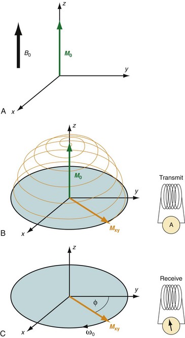
 FIGURE 81-1
where ω0 is referred to as the Larmor frequency, γ is the gyromagnetic ratio of protons (42.58 MHz/T) and B0 is the magnetic field flux of the main field. The precessing transversal magnetization Mxy creates a weak radiofrequency (RF) field that can be recorded with a properly tuned coil (e.g., 63.87 MHz at B0 = 1.5 T) circularly polarized about the axis of precession. As illustrated in Figure 81-1B, the tipping of the net magnetization vector is accomplished with a second RF system that can generate an oscillating magnetic field, B1, close to the resonance frequency, a concept called RF excitation. In practice, the RF pulse is played out very shortly (in the order of milliseconds) and a remarkably small B1 field is sufficient for RF excitation (e.g., ~50 mT in comparison to B0 = 1.5 T).
Multiple RF excitations are needed to acquire enough data for a two-dimensional image. The time between successive excitations is controlled by the MRI parameter repetition time (TR). The time between an RF excitation and the recording of the signal is controlled by the MRI parameter echo time (TE). Both of these parameters have an impact on the measured MR signal because they dictate how much time is allowed for the decay of the transversal magnetization (TE) or the regrowth of the longitudinal magnetization (TR). The actual measured MR signal depends on the T1 and T2 relaxation times, proton density, choice of TR and TE, and other imaging parameters, but also on factors such as motion, diffusion, and temperature. In MRA, the goal is to generate high signal differences between blood and surrounding background tissues, which is achieved by incorporating the motion of the blood using noncontrast MRA techniques or T1 shortening of blood by a circulating Gd chelate contrast agent using CE-MRA. Typical relaxation times are T1/T2 = 1200/250 ms for arterial blood and T1/T2 = 1200/220 ms for venous blood at 1.5 T.2 Whereas T1 increases with field strength for most tissues (1600 ms for arterial blood), the T2 undergoes a small decrease.
Image Encoding
To create an image, the spatial distribution of the protons has to be resolved. Spatial encoding is achieved with the use of spatially and temporally varying magnetic fields. In the first step, the signal-generating volume is reduced to a slice (two-dimensional imaging) or volume (three-dimensional imaging) by selective excitation. A linear magnetic field gradient is superimposed onto the main magnetic field in the slice (or volume) direction simultaneously with the RF excitation. Consequently, the resonance frequency of the spin system is linearly varying as well. The RF system generates a pulse that excites not only a single precession frequency but all the frequencies contained in the desired slice or volume. Spins located outside the desired volume are not excited because their precession frequency is higher or lower than the frequency band covered by the RF excitation. Theoretically, this concept could be repeated in orthogonal directions ultimately to excite only a single point in the object, and then repeat the measurement until all points in the image are sampled. However, a much more efficient approach is Fourier encoding, whereby each sampled signal contains contributions from all spins in the object, therefore dramatically increasing the SNR of the acquisition. Figure 81-2 shows a basic example for a Fourier-encoded two-dimensional acquisition in the form of a pulse sequence diagram that illustrates the timing for RF excitation, the gradients, and data acquisition.
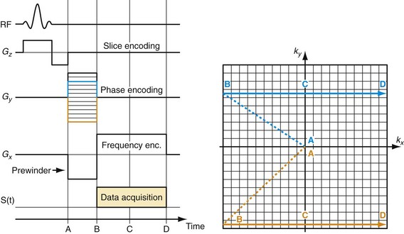
 FIGURE 81-2
The third gradient, called the phase-encoding gradient, is switched on and off prior to the frequency-encoding gradient. This leads to a linearly varying phase of the net magnetization vectors along the direction of that gradient, providing encoding for a single spatial frequency. In other words, with properly controlled gradients, the time-dependent MR signal actually samples the spatial frequencies of the object in two dimensions. Figure 81-2 shows how the sampling trajectory in the spatial frequency space, also called k-space, is controlled by the area under the gradient waveforms.
If that experiment is repeated several times with varying phase-encoding gradients, then multiple spatial frequencies are sampled in the phase-encoding direction as well and an image can be reconstructed via inverse two-dimensional Fourier transform. Figure 81-3 shows an example of a sagittal head scan. The received signal is digitized by an analog to digital converter and a discrete inverse two-dimensional Fourier transform generates the corresponding image, which contains magnitude (length of the transversal magnetization) and phase information (position in the transverse plain in respect to the coil axis) for each voxel. Most MRI relies on the magnitude image only. However, in some applications, such as phase contrast MRA, the phase information plays an essential role in generating image contrast.

 FIGURE 81-3
Figure 81-4 provides some insight about the signal distribution in k-space. For this image, most of the signal energy is located around the origin of k-space. This area defines the weighting for the low spatial frequencies, which define the coarse outline of the imaged object yet lacks information on edges. The broad pattern of the phantom can be identified even with less than 0.5% of the k-space samples from the full-resolution image. However, all the detail is lost, which is defined in the unsampled higher spatial frequencies. The difference in images between the low-resolution images and the fully sampled image reveals the errors caused by limiting the acquisition to lower spatial frequencies only.
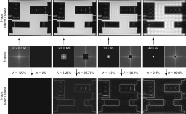
 FIGURE 81-4
The basic signal-to-noise ratio (SNR) in MR acquisitions is given by

where Tacq represents the data acquisition time.3 Based on this relationship, one notes that the desirable properties for MRA, such as small voxel size for higher spatial resolution imaging and short acquisition times for fast scans, are detrimental to the obtainable SNR. Frequently, compromises in scan parameter choices are necessary for optimization of MRA for imaging individual vascular territories, with each offering unique challenges for proper visualization by MRA.
TECHNICAL REQUIREMENTS
Magnetic Resonance Scanner
Each MR scanner is designed to provide a magnetic field, B0, that is homogeneous over the imaging volume, stable over time, and against the influence of external sources. The magnetic induction of the field, also frequently referred to as the magnetic field strength, is measured in tesla (T) or gauss (G), where 1 T = 104 G. The most common modern MR scanners used in clinical practice are whole-body scanners that rely on a superconducting magnet with a field strength of 1.5 or 3 T. For comparison, the field strength of a 1.5-T MR scanner is about 30,000 times stronger than the earth’s magnetic field (~0.5 G). Superconducting MR scanners contain several coils that run in series to form a solenoid and create a cylindrically symmetrical magnetic field, with the main magnetic field aligned with the z-axis of the cylindrical housing (Fig. 81-5). They operate near absolute zero temperature (~4 K, or −270° C) to effectively eliminate electrical resistance in the coil wires, allowing large currents that generate high magnetic fields. Other MR scanner designs include resistive magnetic fields (without superconductivity) that operate at lower magnetic field strengths (<0.15 T), permanent magnetic fields that have intermediate field strength (<0.7 T), smaller bore diameter MR scanners for extremity imaging, and open bore designs (usually <0.7 T) to improve patient comfort and reduce claustrophobia. Imaging at lower field strengths reduces some of the problems encountered at higher fields, such as reduced RF penetration and increased energy absorption. However, MRA applications greatly benefit from imaging at higher field strength because the SNR increases linearly with field strength. MR scanners with field strengths of 3 T are becoming more prevalent in clinical settings and favorable results have been reported with these systems4; more recently, higher field 7-T research MR systems are being investigated.5
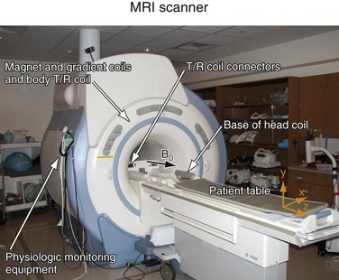
 FIGURE 81-5
Gradient System
The magnetic field gradient system typically consists of three orthogonal gradient coils embedded within the housing of the scanner. Gradient coils are designed to produce a spatially varying magnetic field that can be temporally altered. Although these additional magnetic fields are dramatically smaller than the main magnetic field, they are an essential component for spatial encoding of the signal distribution in the imaging volume of interest. Gradients are rated by their maximum gradient strength (the higher the better) and the time needed to rise to the maximum gradient strength (slew rate—the faster the better). The gradient waveforms in Figure 81-2 are idealized in that they can be switched on and off instantaneously.
Radiofrequency System
The RF system serves the purpose of converting pulsed oscillating currents from a power amplifier into an oscillating magnetic field, also referred to as the B1 field, for the excitation of the nuclear spin system. This is accomplished by a transmitter coil tuned to the resonance frequency of the spin system under investigation. Such coils are designed to provide a uniform B1 field over the imaging volume to ensure uniform spin excitation. So-called birdcage coils are well suited for this purpose and exist as whole-body coils built into the scanner housing and as specialty coils, such as for head or knee imaging (Fig. 81-6).
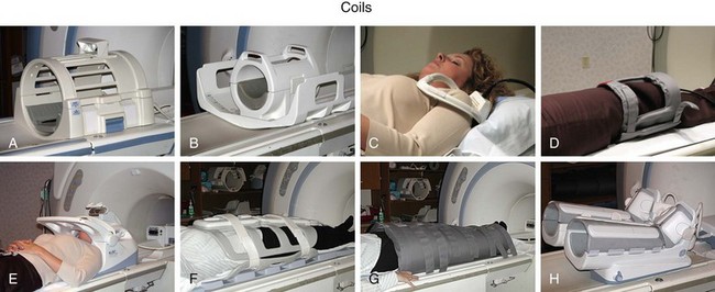
 FIGURE 81-6
A receiver coil is used to detect the RF field created by the precessing magnetization of the nuclear spins after their excitation. The same coil may be used for transmitting and receiving the RF signals, which are referred to as transmit-receive coils (see Fig. 81-6A and B). However, in many applications, it is advantageous to use special local coils that are sensitive only to the signal from the region close to the coil. Such local coils can have a significantly better SNR, as described by equation 2, especially compared with the whole-body transmit-receive coil that encounters noise contributions from the whole volume within it that is much larger than that of smaller local coils. Figure 81-6 shows examples of such local coils, including a shoulder coil (C) and a multipurpose flex coil (D).
Coil arrays consist of multiple local receiver coils to provide a larger coverage with the SNR advantage of local coils. These multielement RF coils have become very common and are available for many applications in many body regions (Fig. 81-6E-H). Figure 81-7 demonstrates the local coil sensitivities of an eight-channel head coil in a three-dimensional TOF MRA and the cumulative image obtained from combining all channels. Data from multiple coils cannot be combined during acquisition and must be stored individually. Therefore, the acquired data size increases linearly with the number of coils, and image reconstruction must be completed for each channel before they can be combined. However, current reconstruction engines are prepared to handle the additional workload for 8 to 16 channels without significant delays.
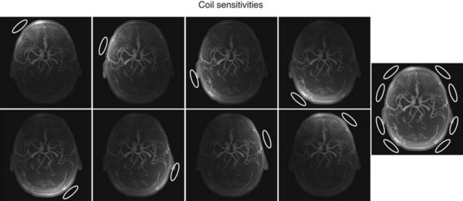
 FIGURE 81-7
Parallel Imaging
More recently, scan time reduction methods were developed that explore the redundancy in the information contained in multiple receiver coils with partly overlapping sensitivity regions. SMASH (simultaneous acquisition of spatial harmonics),6 SENSE (sensitivity encoding),7 and GRAPPA8 are acquisition and reconstruction methods from this group referred to as parallel imaging, which have found rapid commercial adaptation for cardiovascular imaging, especially CE-MRA. With this approach, the equivalent of multiple-phase encoding steps is acquired during a single readout. Although the advantage of accelerated imaging comes at the expense of a reduction in SNR, it can be highly beneficial in situations in which there is sufficient SNR and rapid image acquisition is desired. Basically, all CE-MRA applications fall into this category because faster imaging can improve the frame rate for dynamic acquisitions or reduce breath-hold lengths or other artifacts related to patient motion. As shown in Figure 81-8, attention has to be paid to potential local noise amplifications from the reconstruction process, frequently described as g-factor maps, when using high acceleration factors.
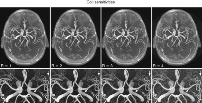
 FIGURE 81-8
The scan time reduction factor that can be obtained with parallel imaging depends on the number of independent coil elements and their arrangement. Therefore, further increases in the number of coil elements and receiver channels promise even greater reductions in scan time. Consequently, the recent progress in parallel imaging has led to renewed interest in coil design and receiver systems. New MRI platforms provide the ability to connect many coil elements and acquire the signal from as many as 16 to 32 receivers simultaneously and systems with even more channels are being explored. With higher receiver coil counts, the SNR and coverage can be further improved or higher acceleration factors can possibly be obtained. Current design problems, such as with the decoupling of individual coil elements, has limited commercial coil designs to 8 to 32 elements. In research settings, systems with up to 128 receiver channels have been recently evaluated and demonstrated regional SNR benefits and high acceleration factors for cardiovascular applications as compared with lower count coil arrays.9 However, the lack of penetration for small coils might limit additional benefits for regions of interest that are more distant from the body surface. It remains to be seen at which point additional coil elements are still beneficial, especially when the noise in the MR system becomes dominated by electrical noise from the receiver system, instead of intrinsic noise contributions caused by random motion of electrons in the patient’s tissue.
Power Injector
For CE-MRA, a Gd-based contrast agent is injected intravenously, usually into an antecubital vein. The injection of the contrast agent is followed by the injection of sterile saline to flush the contrast material out of the delivery system and ensure that the contrast bolus is sufficiently central within the body. Although manual injections are possible, the use of a computer-controlled, MR-compatible power injector is usually preferred. The power injector is more precise in delivering reproducible injection rates and its use omits the need for an operator in the scan room during imaging. Power injectors also provide features to assist in dynamic timed studies and breath-hold maneuvers and allow for multiphase injections. A typical system consists of a delivery component in the scan room and a user console in the operator room (Fig. 81-9). Manual injections have the advantage that the physician is right next to the patient and can better monitor the administration of contrast agent and the status of the patient.
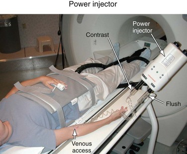
 FIGURE 81-9
TECHNIQUES
Contrast-Enhanced Magnetic Resonance Angiography
CE-MRA10 has gained widespread clinical acceptance because of its ability to provide diagnostic angiographic data sets very quickly and reliably. In many practices, CE-MRA has replaced conventional x-ray angiography as the preferred method for angiographic depiction of specific anatomic regions such as the aorta, carotid arteries, and peripheral arteries.
The exposure to gadolinium-based contrast material has been associated with the development of nephrogenic systemic fibrosis (NSF).11 Patients with compromised kidney function are at risk and proper screening (knowledge of the patient’s renal function—estimated glomerular filtration rate [GFR] and serum creatinine level) is important to minimize potential risks. A more detailed discussion of NSF can be found in Chapter 18.
The MR signal in CE-MRA is dominated more by the T1-shortening effect of the blood signal caused by the presence of the circulating contrast agent and less by signal properties related to flowing blood. CE-MRA, in essence, provides a lumenogram similar to that of conventional x-ray angiography or CTA. T1 weighting is achieved with spoiled gradient echo pulse sequences with small flip angles and short TE and TR values. Short repetition times leave little time for signal regrowth between successive excitations and form the basis for good background suppression. Therefore, only tissues with a short T1 time will generate significant signal contributions (Fig. 81-10). A pitfall of this technique is its application in regions of the body where there is an abundance of fat in the surrounding background tissue. In these cases, the signal of surrounding fat may diminish the apparent contrast-to-noise discrimination of the arterial segments from signal of surrounding fat. Fat suppression or image subtraction of precontrast mask data sets can be used to improve the depiction of arteries on CE-MRA in such cases.
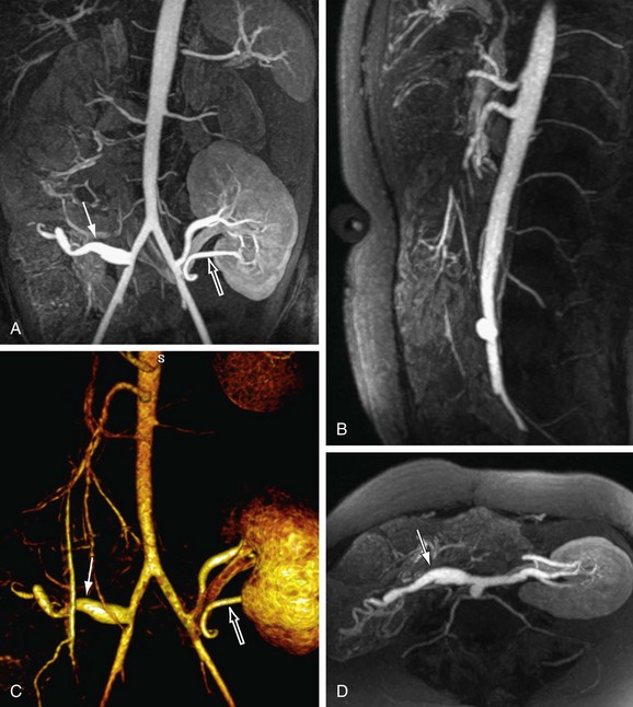
 FIGURE 81-10
Bolus Timing for Contrast-Enhanced Magnetic Resonance Angiography
To optimize image quality, the data acquisition has to be synchronized with the contrast bolus transit through the target vasculature, which is typically arterial. The imaging objective is thus to capture critical image data during the arterial first passage of the bolus prior to contrast bolus progression and signal enhancement of the veins, and prior to significant dilution of the contrast bolus within the arterial tree (Fig. 81-11). Several approaches have been proposed to acquire the data during peak arterial Gd concentration so that a high SNR image without venous contamination is obtained. The simplest way to estimate the arrival time of the bolus is the best guess technique. However, this is also a highly inaccurate technique because the arrival time depends on a variety of parameters, such as the patient’s cardiac output, size, and underlying vascular pathology.
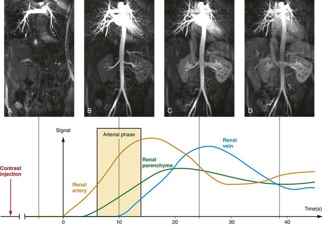
 FIGURE 81-11
Contrast bolus arrival time can be determined for an individual patient by performing a preliminary timing scan with a low dose of contrast agent (e.g., a 1- to 2-mL Gd chelate contrast agent test bolus).12 With this method, a series of two-dimensional images of the target arterial tree is rapidly acquired (typically about one image/sec) and analyzed for arrival time of the test bolus into the artery under investigation. Based on these images, the arrival time for a full injection is predicted and a suitable delay time for the start of the data acquisition is determined. Disadvantages of the technique include a prolonged examination time for two injections and the use of additional contrast agent, which will necessarily increase the signal contributions of adjacent background tissues and the urinary system. Also, the arrival time of the contrast may vary because of differences in breathing or the initiation of a breath-hold.
Another timing method is to integrate an automated detection scheme that can monitor the signal in an arterial voxel13 or a near–real-time two-dimensional image display (MR fluoroscopy) of the region of interest14 that can be used to monitor for contrast bolus arrival and initiate the scan on arrival of the contrast bolus. These latter techniques have the advantage of a single injection for the CE-MRA itself and thus improved background signal suppression.
Magnetic Resonance Angiography Scan Time
Another consideration for CE-MRA is overall scan time for image acquisition. As noted, the duration of preferential arterial enhancement by the contrast bolus provides the ideal imaging window for CE-MRA. In some cases, such as with the carotid arteries, this window can be as brief as 5 seconds. Moreover, CE-MRA in the body is often improved if performed during a breath-hold because respiratory motion can result in significant blurring on CE-MRA. These time constraints limit the maximal achievable spatial resolution for a given three-dimensional MRA acquisition. For example, if one wants to acquire a cubic volume with an isotropic spatial resolution of 256 voxels in each dimension (Fig. 81-12A) and a typical TR of 5 ms, then the total scan time would be Tscan = TR × Ny × Nsl = 328 sec, where Ny and Nz represent the number of phase encoding steps in y and z. Instead, a reduced data set is sampled to limit the scan duration to 10 to 30 seconds, either with compromised spatial resolution by symmetrical k-space reduction (see Fig. 81-12B), reduced coverage (see Fig. 81-12C), asymmetrical reductions in k-space that maintain the spatial resolution by exploring symmetries in k-space (see Fig. 81-12D),15 reduction of phase encoding steps with parallel imaging (see Fig. 81-12E),6–8 or a combination of these techniques in a single- or double-phase encoding direction.
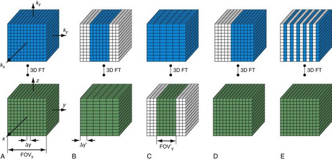
 FIGURE 81-12
K-Space View Ordering
If it were possible to extend the scan time beyond the period of preferential arterial enhancement (i.e., arterial phase) without signal from the veins, the obtainable spatial resolution could be improved. To this end, sampling schemes have been developed that tailored the temporal order of the phase-encoding steps to optimize image quality. Because the central spatial frequencies (i.e., central k-space data) define the image contrast, it is necessary to acquire these portions of k-space during the peak of the arterial signal intensity, before the bolus arrives in the veins.16 Higher spatial frequencies that dominate the edge information of an image (i.e., peripheral k-space data) can be acquired even after venous contamination to provide the desired spatial resolution with minimal signal interference from venous structures.
In traditional three-dimensional MR acquisition schemes, sequential phase-encoding schemes are applied (Fig. 81-13A). The first acquired view in such a scheme is the most distant from the origin of k-space. Line after line of k-space is acquired linearly by advancing one phase encode (here, kz) from its minimum to its maximum, while the other phase encode is kept constant (here, ky). However, this scheme is not well suited to ensure sampling of the central k-space region during peak arterial enhancement. To this end, centric view-encoding k-space schemes were developed whereby the views near the k-space origin are acquired during the initial period of the scan. Centric view encoding k-space schemes facilitate better synchronization of key central k-space image data acquisition with the arrival of the contrast bolus. One such implementation is linear centric view encoding (see Fig. 81-13B), in which the views are ordered in a double loop; the outer one (here, ky) is ordered based on its distance from the origin (+Δky, −Δky, +2Δky, −2Δky,…) whereas the inner loop (here, kz) is still chosen sequentially. A further optimized variation of this scheme is the so-called elliptical centric view ordering.17 In this approach, the temporal order of the acquisition of k-space lines is determined by their distance in the ky-kz plane to the center of k-space, providing a more compact and true centric encoding in both phase-encoding dimensions. The larger the distance between a k-space point and the origin, the later that particular kx line is sampled (see Fig. 81-13C). When properly timed, such ordering allows for the acquisition of the central k-space data during the signal intensity peak in the arteries and the higher spatial frequencies thereafter. It is also more robust to artifacts generated by the modulation of the contrast concentration and suppression of motion artifacts.18 An example of such an acquisition is shown in Figure 81-10, demonstrating the large coverage, high spatial resolution, and three-dimensional reformatting capabilities of a CE-MRA data set acquired in a single breath-hold. Elliptical centric view ordering is particularly helpful for imaging arterial territories such as the carotid arteries, which can have especially brief periods of preferential arterial enhancement.
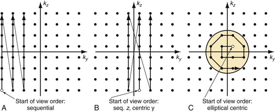
 FIGURE 81-13
Time-Resolved Contrast-Enhanced Magnetic Resonance Angiography
In keyhole imaging, the acquisition process is split into a dynamic phase, in which central k-space data are acquired rapidly but with limited spatial resolution, and a subsequent second phase, whereby the missing high spatial frequency data (i.e., peripheral k-space data) is acquired to provide image detail.18,19 These two acquisitions are then combined to generate a dynamic series with high spatial and high temporal resolution by updating only the central k-space region (Fig. 81-14). The underlying assumption is that most of the signal changes are reflected in the central k-space region (see Fig. 81-4). The drawback of the approach is the missing dynamic information about high spatial frequencies. Dynamic information is captured only with low spatial resolution whereas the high spatial frequency data, which define finer structures such as smaller vessels, are acquired only once and shared across the acquisition. If the relevant information under investigation contains changes in the outer portions of k-space, then keyhole imaging can produce images with an erroneous time course.20
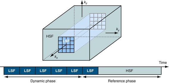
 FIGURE 81-14
Another commercially available approach, three-dimensional TRICKS, also shares data among time frames but does not update the central region alone. In three-dimensional TRICKS (three-dimensional time-resolved imaging of contrast kinetics) imaging,21 k-space is divided into subvolumes based on their distance to the center of k-space. Figure 81-15 shows an implementation of TRICKS with an elliptical centric view ordering scheme whereby the phase- and slice-encode ordering is based on their distance in the ky-kz plane from the center of k-space. In this figure, the subvolumes consist of a cylinder for the region containing lower spatial frequencies (A) and cylindrical shells of equal volume for the regions representing higher spatial frequencies (B and C). In practice, most examinations are acquired with a decreased spatial resolution in the slice-encoding direction, z, for a decreased imaging time and higher SNR. In this case, the higher spatial frequency regions become incomplete cylindrical shells. The central region, A, contains the low spatial frequency information and is sampled every second time frame, whereas regions B and C are sampled every fourth time frame only. For each newly sampled k-space subvolume, a complete k-space volume is assembled by temporal interpolation of the adjacent subvolumes acquired before, during, and after the current time frame.
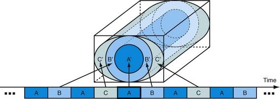
 FIGURE 81-15
This approach continuously acquires data during the passage of the contrast agent and is relatively insensitive to variation in timing and shape of the contrast bolus. An example for an examination of the abdominal and pelvic vasculature is shown in Figure 81-16. The maximum intensity projection (MIP) images represent reformats of three-dimensional volumes reconstructed for each time frame.
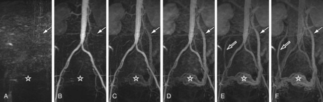
 FIGURE 81-16
Mask Mode Subtraction
Figure 81-17 shows an example of mask mode subtraction for an examination of the pelvis. Mask mode subtraction is extremely beneficial when using multiple injections of a Gd chelate contrast agent because the accumulated effects of prior contrast administration can be minimized by the use of imaging subtraction. With this method, time-varying background signals caused by patient motion or motion of the gastrointestinal tract are not affected. Although the contrast in the images is improved by mask mode subtraction, the actual SNR is decreased by  , because the noise of the two images is additive.
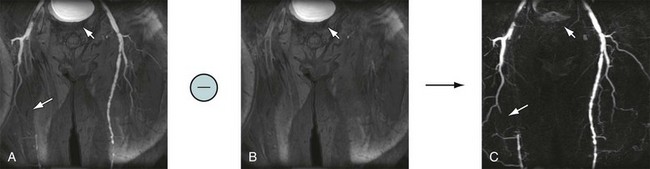
 FIGURE 81-17
Time-of-Flight Magnetic Resonance Angiography
Image contrast in TOF MRA relies on the inflow of blood into the imaging slice so that the signal from moving blood is brighter than that from stationary tissue. Because TOF MRA is inflow dependent, it is best suited for vascular territories that allow for slice orientations with pronounced inflow effects, such as the lower extremities or carotid arteries, which have straight vessel paths and little in-plane flow. As a non–CE-MRA technique, TOF MRA provides an alternative to CE-MRA in patients with contraindications to Gd chelate contrast agents. It is routinely used for cranial MRA, providing spatial resolution and image quality superior to CE-MRA because the scan time is not limited to an arterial-venous window (Fig. 81-18). However, in vessels with more tortuous pathways with in-plane components and slow flow, TOF MRA acquisitions can suffer from disease-mimicking signal voids.
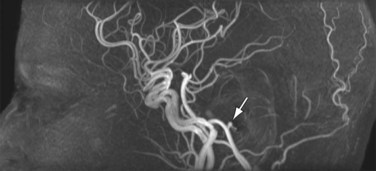
 FIGURE 81-18
Two-Dimensional Time-of-Flight
The TOF acquisition strategy aims to saturate partially the longitudinal magnetization of nonmoving spins so that unaffected moving spins appear bright in comparison.22 Similar to CE-MRA, a spoiled gradient echo sequence is used to achieve this goal. With this acquisition, the repeated RF pulses used for excitation in the beginning of each TR diminish the available longitudinal magnetization until an equilibrium between signal regrowth from relaxation and signal decrease from the RF excitation is reached (Fig. 81-19). The actual signal depends on the TR, the T1 of the tissue, and the flip angle. In two-dimensional TOF imaging, the imaging slice is oriented perpendicular to the flow direction. Stationary tissue experiences all RF pulses and will only have small signal contributions in the resulting image. However, only a few RF excitations will affect flowing blood as it enters the imaging slice, resulting in a relatively high signal contribution in the angiogram. The longer the blood stays in the imaging slice, the more the signal differences diminish. Consequently, the vessel to background contrast decreases as the slice thickness increases or the velocity of blood flow decreases. A longer TR will increase the vascular signal but will also increase the signal from background tissues and lengthen the scan time. Therefore, intermediate TR times are usually chosen. An increased flip angle will decrease the signal contribution from stationary tissues, but signal from blood that undergoes multiple RF excitations will also decrease (see Fig. 81-19). Therefore, intermediate flip angles are used for most clinical applications.
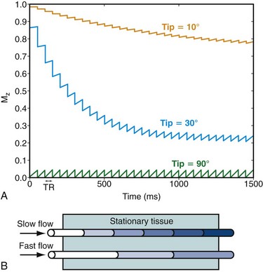
 FIGURE 81-19
Without any further modifications, arterial and venous blood flow will cause a bright signal in TOF angiograms. In most applications, it is desirable to image selectively the arteries or veins only. This can be easily achieved with the use of saturation bands in vascular regions with arterial and venous flow in opposing directions.23 With this approach, a saturation pulse is applied parallel to the imaging slice to eliminate unwanted inflow signal from a particular direction. Figure 81-20 demonstrates an example of arterial and venous suppression in an axial slice through the neck with the use of superior and inferior saturation slabs.
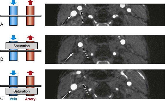
 FIGURE 81-20
Volume data can be achieved with two-dimensional TOF MRA whereby a series of contiguous two-dimensional slices are acquired sequentially over the vascular territory of interest. In most cases, two-dimensional TOF MRA is accompanied by a saturation band (e.g., inferior saturation band for lower extremity arterial imaging) that is applied sequentially with each two-dimensional slice, a feature also known as a walking saturation band. This approach is commonly used in TOF examination of the lower extremities in which coverage of the vessels from the pelvis to the feet is achieved with sets of axial slices that are acquired over multiple stations (Fig. 81-21). TOF examinations in the abdomen, pelvis, and lower extremities typically must be cardiac gated because of the flow pulsatility that can result in significant fluctuations in arterial signal and artifacts. The acquisition of central k-space data during systole optimizes arterial inflow signal on TOF MRA.
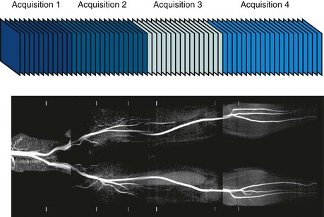
 FIGURE 81-21
Three-Dimensional Time-of-Flight
In three-dimensional TOF MRA,24 the SNR is improved compared with sequential two-dimensional TOF because all the magnetization in the excited volume contributes to the signal of each sampled data point. In addition, the slice encoding for thin slices less than 1 mm thick, with reasonable echo times for artifact suppression, poses major challenges to two-dimensional TOF but can easily be achieved with three-dimensional TOF. The phase-encoding steps and not the slice-encoding gradient determine the slice thickness in three-dimensional TOF. The increased spatial resolution reduces intravoxel dephasing and permits the visualization of smaller vessels that otherwise might be obscured by partial voluming effects.
Sequential Three-Dimensional Time-of-Flight
The signal loss of flowing blood from saturation in a thick three-dimensional volume can be reduced by exciting smaller volumes. The use of MOTSA (multiple overlapping thin slab angiography)25 provides large coverage with thin slabs (i.e., thin volumes), thereby combining benefits from two-dimensional (reduced blood saturation) and three-dimensional TOF (small voxels, high SNR, and short TE). Overlapping of the thin slabs reduces artifacts from slab profiles and partial saturation, making this approach the method of choice for cranial and carotid MRA, in which high spatial resolution is essential (Fig. 81-22A; see Figs. 81-7 and 81-18). Such volumetric acquisitions benefit from ramped flip angles designed to counteract the signal loss from partial saturation effects when blood moves through the imaging volume. A lower flip angle, in which the arterial blood enters the imaging volume, and a higher flip angle, in which the arterial blood leaves the imaging slice, provide a homogeneous vessel signal across the imaging volume (see Fig. 81-22B). The linearly varying flip angle reduces saturation effects for the blood entering the volume and increases the signal for the blood leaving the volume. The amplified saturation of blood exiting the volume is inconsequential because it will not be used for signal generation once it has left the imaging volume.
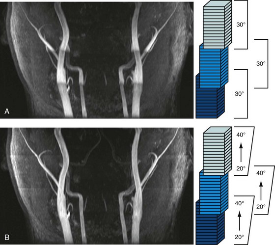
 FIGURE 81-22 Volumetric TOF acquisition with MOTSA (multiple overlapping thin slab angiography).24 This neck examination was acquired with three partially overlapping thin slabs to provide large coverage with thin slices, high SNR, and good vessel contrast. A, When a constant flip angle of 30 degrees is used, the vessel signal decreases as the arterial blood travels supine and experiences additional RF pulses (arrows). B, The homogeneity of the vessel signal can be further improved with ramped flip angles to counteract this effect.
(Courtesy of Dr. Frank R. Korosec, University of Wisconsin-Madison, Madison, Wis.)
Phase Contrast Magnetic Resonance Angiography
Phase contrast MRA (PC MRA) provides quantitative velocity and flow measurements in vascular territories throughout the body and, like TOF, can be acquired in two-dimensional or three-dimensional modes. Two-dimensional PC MRA is commonly used in an ECG-gated cine mode for the dynamic assessment of cardiac valve function, pulmonary and systemic flow, and unusual shunt determinations in patients with congenital heart disease. In addition, MR angiograms can be derived from the acquired data, making this approach another alternative to CE-MRA in patients who cannot be given Gd chelate contrast agents. PC MRA works well for two-dimensional projections through thick sections and, compared with TOF methods, smaller vessels with low blood velocities can be identified. PC MRA is also particularly good when performed following the administration of Gd chelate contrast agents and is a good alternative when the initial CE-MRA scan is nondiagnostic.26
Whereas the imaging contrast between blood and surrounding tissues in all other MRA techniques is based on the magnitude of the magnetization, PC MRA uses bipolar gradients for phase manipulation of the magnetization.27 Figure 81-23 demonstrates how the gradient pair causes the phase of stationary spins to accumulate to zero, whereas spins that move along the axis of the gradient accumulate a net phase proportional to their velocity. Because MR images contain unpredictable phase contributions from magnetic susceptibilities, eddy currents, measurement imperfections, and other sources, a reference image without velocity encoding has to be acquired. On subtraction of the reference phase from the velocity-encoded image, these local phase offsets are removed. Therefore, one-directional velocity encoding requires the acquisition of two images, thereby doubling the scan time. In the phase difference image, the signal in each voxel is linearly proportional to its velocity. Blood moving along one direction of the gradient axis is assigned a bright (white) signal and blood moving along the opposite direction is assigned a dark (black) signal. PC acquisitions, therefore, can provide directional information of blood flow. A magnitude image is also reconstructed as the average of the two acquisitions to provide anatomic information. The velocity-encoding direction can be perpendicular to the imaging plane (through-plane flow) or in plane in the phase or frequency direction. For pulsatile flow measurements, cine PC imaging with ECG gating28 is performed to capture the flow dynamics for multiple time points within the cardiac cycle. Because of the slower acquisition speed of MRI , data sampling for cine series stretches over multiple heartbeats. Reductions in scan time because of high-performing gradients (shorter TR) and parallel imaging can improve the temporal and spatial resolution achievable for cine PC imaging within a patient-friendly breath-hold duration. Figure 81-24 shows a magnitude image and several phase difference images at peak systolic flow for an oblique imaging plane in a chest that was oriented perpendicularly to the path of the ascending aorta with through-plane velocity encoding.
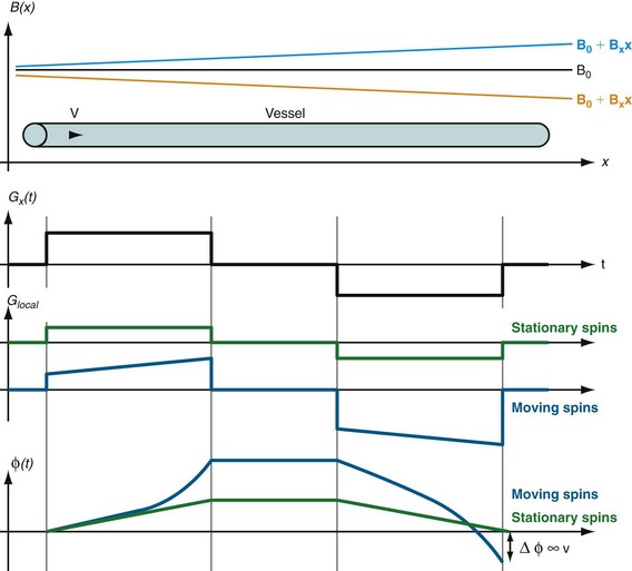
 FIGURE 81-23
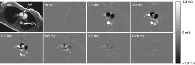
 FIGURE 81-24
The application of bipolar gradients along a second and third gradient axis extends the technique to two-dimensional and three-dimensional flow encoding. The same reference image can be used for calculating the directional phase differences, yet the total scan time is prolonged to three or four acquisitions, respectively. Figure 81-25 shows an example of three-directional velocity encoding for a slice covering the aortic arch. The different in-plane and through-plane components of the velocity vector can be appreciated as three gray-scale images. The concept can be further extended to volumetric cine imaging,29 thereby providing comprehensive information on the anatomy and velocity fields over a vascular territory.
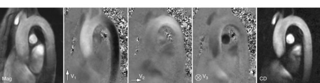
 FIGURE 81-25
Figure 81-26 shows an example of an axial imaging slice in the neck with optimized Venc settings for arterial flow analysis (50 cm/sec) and cerebrospinal fluid (CSF) flow analysis (5 cm/sec) and an intermittent Venc of 30 cm/sec. In practice, the bipolar gradient waveform is automatically calculated from a user input on the desired Venc based on reference velocities for normal vessels or expected velocity ranges. Ideally, the Venc is set slightly above the peak velocity within the vessel of interest. However, peak velocity, especially in diseased vessels, may be difficult to predict, and the PC acquisition may need to be repeated at a more appropriate Venc setting if the initial Venc setting is suboptimal.
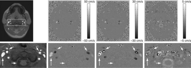
 FIGURE 81-26
Several factors lead to an increased susceptibility of PC MR to intravoxel dephasing:
Postprocessing
In addition to the magnitude and phase image, complex difference (CD) images can be derived from PC acquisitions. The complex difference image is obtained as the length of the vector obtained by complex subtraction of the velocity-encoded data from the reference data, thereby incorporating phase and magnitude into the calculation. As opposed to phase difference images, complex difference images are non-negative and do not suffer from discontinuities from velocity aliasing. As shown in Figure 81-25, they are well suited for the display of vessel paths with good background suppression, but do not provide quantitative or directional flow information.

where Qvoxel is given in mL/min, velocity is determined using the phase map images (cm/sec), and area is given by the spatial resolution of the phase map (cm2). The flow rate through a vessel is simply determined by integration over a manually or semiautomatically defined cross-sectional ROI that encompasses the vessel circumference. Flow volumes throughout the cardiac cycle can be calculated by integration over the sampled time points, as shown in the valve analysis in Figure 81-27.
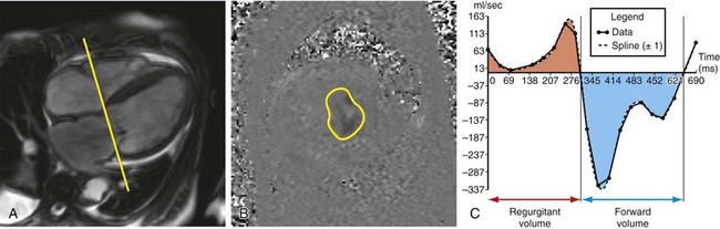
 FIGURE 81-27
Flow analysis and visualization for cine three-directional volumetric velocity mapping has gained significant interest but is currently limited to research applications, partly because of the lack of intuitive analysis platforms. Advanced visualization techniques such as particle tracers, streamlines, and velocity vectors are limited to specialized software platforms (Fig. 81-28). However, the availability of comprehensive information on cardiovascular anatomy and function from a single examination is appealing and possibly allows for the derivation of additional hemodynamic parameters, such as trans-stenotic pressure gradients and wall shear stress within the limits of the spatial resolution of the acquisition. Without taking advantage of accelerated imaging methods, the total scan time for such measurements, Tscan, becomes prohibitively long:
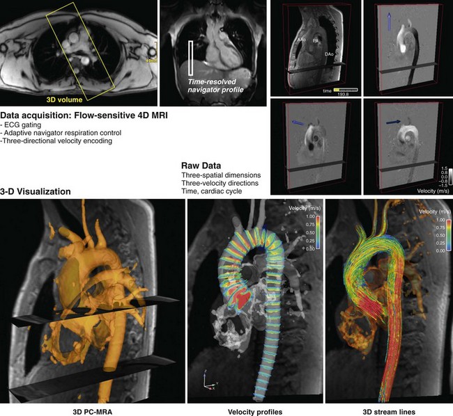
 FIGURE 81-28
where NFD = no. of flow-encoding directions, NPE = no. of phase-encoding directions, NSE = no. of slice-encoding directions, TR = repetition time, and TR = no. of cardiac phases. Similar to CE-MRA, accelerated PC imaging approaches include partial Fourier acquisitions, view sharing and temporal interpolation schemes, and use of parallel imaging techniques.
Steady-State Free Precession Magnetic Resonance Angiography
In balanced steady-state free precession (SSFP) imaging, the magnetization is manipulated so that both the transverse and the longitudinal components reach a steady state and contribute to the MR signal. The clinical adaptation of this imaging approach, also known as true fast imaging with steady-state precession (trueFISP), fast imaging employing steady-state acquisition (FIESTA), and balanced fast field echo (bFFE), had been delayed until recent hardware improvements, particularly in gradient performance and field shimming, minimized, image-degrading artifacts. This sequence is extensively used for the evaluation of cardiac function.31
Whereas the image contrast in the rapid spoiled gradient echo sequence depends mostly on T1-dependent and inflow effects for a high blood signal, SSFP provides an inherently high steady-state signal for species with a large T2/T1 ratio, such as in blood. This property explains its extensive use in the evaluation of cardiac function, with striking contrast between the blood pool and the myocardium. However, not only blood has a large T2/T1 ratio, and the challenge for SSFP MRA applications becomes the suppression of unwanted signals, particularly from fat and veins. Fat suppression is usually accomplished with water-selective excitation pulses or repeated spectral fat saturation pulses. Figure 81-29 shows MRA scans of the thoracic aorta acquired with an SSFP sequence and fat suppression.
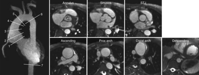
 FIGURE 81-29
In SSFP MRA, data are acquired with very short TR times (~3 ms), allowing for breath-held ECG-gated acquisitions. This approach is becoming a promising alternative for patients with contraindications to CE-MRA with Gd chelate contrast agents. Several modified acquisition schemes have been suggested to improve signal suppression from fat and veins, including the use of arterial spin labeling or saturation bands similar to the ones used in TOF imaging for the suppression of venous signal and slab-selective spin inversions.2 Future clinical evaluations are needed to assess their reliability over a broad patient base. It must also be noted that signal on SSFP MRA is good after the administration of Gd chelate contrast agents and provides an additional imaging option following CE-MRA if specific regions need reassessment.32
Black Blood Imaging
One final technique, black blood imaging, requires specific mention, because it also can be used for the depiction of blood vessels. With black blood imaging techniques, the stationary tissue produces a signal with high amplitude, whereas the signal from moving spins is nulled.33 This is the reverse of all other MRA techniques described here, which result in bright vascular signals. Black blood methods are based on spin-echo sequences with long TR times. The most common approach for generating this contrast is by the use of a black blood pulse consisting of two consecutive 180-degree excitation pulses (double-inversion recovery fast spin echo [DIR FSE]). The first pulse is a non–slice-selective pulse that effectively inverts the magnetization in the excitation volume of the transmit coil. As a result, the initial value of the normalized longitudinal magnetization is not 0, as is the case for a 90-degree excitation, but −1. The second pulse is selective to the magnetization of protons in the imaging slice, basically reversing the previous inversion. However, the protons outside the imaging slice are not affected by the second inversion pulse. Therefore, they undergo T1 relaxation to return to their equilibrium state (Fig. 81-30). The magnetization of blood entering the imaging slice will undergo the same relaxation and its image signal can be nulled when the data acquisition is synchronized with the zero crossing of the longitudinal magnetization. The acquisitions are usually based on fast spin-echo sequences with cardiac gating to allow for imaging with long TRs, ensuring the proper regrowth of the longitudinal magnetization prior to the next excitation.
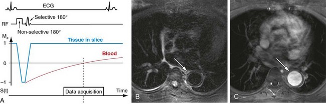
 FIGURE 81-30
Black blood imaging is of value whenever high contrast between the vessel lumen and vessel wall is desired and is typically performed as a two-dimensional acquisition. This technique is particularly useful for imaging atherosclerotic plaque, vasculitis, coronary arteries, and cardiac and intravascular masses and clots (see Fig. 81-30). Furthermore, non–contrast-enhanced MRA sequences that rely on bright blood signal can suffer from signal dephasing in areas of complex flow, resulting in the overestimation of stenoses. Black blood sequences do not suffer from this artifact because the acquisition is designed to provide no signal from within the lumen and can serve as a good adjunct to bright blood MRA for vascular diagnosis. However, drawbacks of this approach include insufficient contrast in regions with low signal intensity background, such as air and bone, and persistent signals in vessels with slow or recirculating blood.


Larkman DJ, Nunes RG. Parallel magnetic resonance imaging. Phys Med Biol. 2007;52:R15-R55.
Lotz J, Meier C, Leppert A, Galanski M. Cardiovascular flow measurement with phase-contrast MR imaging: basic facts and implementation. Radiographics. 2002;22:651-671.
Montgomery ML, Case RS. Magnetic resonance imaging of the vascular system: a practical approach for the radiologist. Top Magn Reson Imaging. 2003;14:376-385.
Paschal CB, Morris HD. K-space in the clinic. J Magn Reson Imaging. 2004;19:145-159.
Rohrer M, Geerts-Ossevoort L, Laub G. Technical requirements, biophysical considerations and protocol optimization with magnetic resonance angiography using blood-pool agents. Eur Radiol. 2007;17(Suppl 2):B7-B12.
Shetty AN, Bis KG, Shirkhoda A. Body vascular MR angiography: using two-dimensional and three-dimensional time-of-flight techniques. Concepts Magn Reson. 2000;12:230-255.
Willinek WA, Schild HH. Clinical advantages of 3.0 T MRI over 1.5 T. Eur J Radiol. 2008;65:2-14.
Wilson GJ, Hoogeveen RM, Willinek WA, et al. Parallel imaging in MR angiography. Top Magn Reson Imaging. 2004;15:169-185.
Wright GW. Magnetic resonance imaging. IEEE Signal Process. 1997;14:56-66.
Zhang H, Maki JH, Prince MR. three-dimensional contrast-enhanced MR angiography. J Magn Reson Imaging. 2007;25:13-25.
1 Nitz WR. MR imaging: acronyms and clinical applications. Eur Radiol. 1999;9:979-997.
2 Miyazaki M, Lee VS. Nonenhanced MR angiography. Radiology. 2008;248:20-43.
3 Macovski A. Noise in MRI. Magn Reson Med. 1996;36:494-497.
4 Gibbs GF, Huston J3rd, Bernstein MA, et al. Improved image quality of intracranial aneurysms: 3.0-T versus 1.5-T time-of-flight MR angiography. Am J Neuroradiol. 2004;25:84-87.
5 von Morze C, Xu D, Purcell DD, et al. Intracranial time-of-flight MR angiography at 7T with comparison to 3T. J Magn Reson Imaging. 2007;26:900-904.
6 Sodickson DK, Manning WJ. Simultaneous acquisition of spatial harmonics (SMASH): fast imaging with radiofrequency coil arrays. Magn Reson Med. 1997;38:591-603.
7 Pruessmann KP, Weiger M, Scheidegger MB, et al. SENSE: sensitivity encoding for fast MRI. Magn Reson Med. 1999;42:952-962.
8 Griswold MA, Jakob PM, Heidemann RM, et al. Generalized autocalibrating partially parallel acquisitions (GRAPPA). Magn Reson Med. 2002;47:1202-1210.
9 Schmitt M, Potthast A, Sosnovik DE, et al. A 128-channel receive-only cardiac coil for highly accelerated cardiac MRI at 3 Tesla. Magn Reson Med. 2008;59:1431-1439.
10 Prince MR, Yucel EK, Kaufman JA, et al. Dynamic gadolinium-enhanced three-dimensional abdominal MR arteriography.J. Magn Reson Imaging. 1993;3:877-881.
11 Thomsen HS, Morcos SK, Dawson P. Is there a causal relation between the administration of gadolinium based contrast media and the development of nephrogenic systemic fibrosis (NSF)? Clin Radiol. 2006;61:905-906.
12 Earls JP, Rofsky NM, DeCorato DR, et al. Breath-hold single-dose gadolinium-enhanced three-dimensional MR aortography: usefulness of a timing examination and MR power injector. Radiology. 1996;201:705-710.
13 Foo TKF, Saranathan M, Prince MR, Chenevert TL. Automated detection of bolus arrival and initiation of data acquisition in fast, three-dimensional, gadolinium-enhanced MR angiography. Radiology. 1997;203:275-280.
14 Wilman AH, Riederer SJ, Huston J, et al. Arterial phase carotid and vertebral artery imaging in three-dimensional contrast-enhanced MR angiography by combining fluoroscopic triggering with an elliptical centric acquisition order. Magn Reson Med. 1998;40:24-35.
15 McGibney G, Smith MR, Nichols ST, Crawley A. Quantitative evaluation of several partial Fourier reconstruction algorithms used in MRI. Magn Reson Med. 1993;30:51-59.
16 Maki JH, Prince MR, Londy FJ, Chenevert TL. The effects of time varying intravascular signal intensity and K-space acquisition order on three-dimensional MR angiography image quality. J Magn Reson Imaging. 1996;6:642-651.
17 Wilman AH, Riederer SJ. Performance of an elliptical centric view order for signal enhancement and motion artifact suppression in breath-hold three-dimensional gradient echo imaging. Magn Reson Med. 1997;38:793-802.
18 Jones RA, Haraldseth O, Muller TB, et al. K-space substitution: a novel dynamic imaging technique. Magn Reson Med. 1993;29:830-834.
19 van Vaals JJ, Brummer ME, Dixon WT, et al. Keyhole method for accelerating imaging of contrast agent uptake. J Magn Reson Imaging. 1993;3:671-675.
20 Bishop JE, Santyr GE, Kelcz F, Plewes DB. Limitations of the keyhole technique for quantitative dynamic contrast-enhanced breast MRI. J Magn Reson Imaging. 1997;7:716-723.
21 Korosec FR, Frayne R, Grist TM, Mistretta CA. Time-resolved contrast-enhanced three-dimensional MR angiography. Magn Reson Med. 1996;36:345-351.
22 Wehrli FW, Shimakawa A, Gullberg GT, MacFall JR. Time-of-flight MR flow imaging: selective saturation recovery with gradient refocusing. Radiology. 1986;160:781-785.
23 Felmlee JP, Ehman RL. Spatial presaturation: a method for suppressing flow artifacts and improving depiction of vascular anatomy in MR imaging. Radiology. 1987;164:559-564.
24 Dumoulin CL, Souza SP, Walker MF, Wagle W. Three-dimensional phase contrast angiography. Magn Reson Med. 1989;9:139-149.
25 Parker DL, Yuan C, Blatter DD. MR angiography by multiple thin slab three-dimensional acquisition. Magn Reson Med. 1991;17:434-451.
26 Hood MN, Ho VB, Corse WR. Three-dimensional phase-contrast magnetic resonance angiography: A useful clinical adjunct to gadolinium-enhanced three-dimensional renal magnetic resonance angiography? Milit Med. 2002;167:343-349.
27 Moran PR. A flow velocity zeugmatographic interlace for NMRI in humans. Magn Reson Imaging. 1982;1:197-203.
28 Nayler GL, Firmin DN, Longmore DB. Blood flow imaging by cine magnetic resonance. J Comput Assist Tomogr. 1986;10:715-722.
29 Wigstrom L, Sjoqvist L, Wranne B. Temporally resolved three-dimensional phase-contrast imaging. Magn Reson Med. 1996;36:800-803.
30 Haacke EM, Lenz GW. Improving MR image quality in the presence of motion by using rephasing gradients. AJR Am J Roentgenol. 1987;148:1251-1258.
31 Carr JC, Simonetti O, Bundy J, et al. Cine MR angiography of the heart with segmented true fast imaging with steady-state precession. Radiology. 2001;219:828-834.
32 Foo TK, Ho VB, Marcos HB, et al. MR angiography using steady-state free precession. Magn Reson Med. 2002;48:699-706.
33 Jara H, Barish MA. Black-blood MR angiography. Techniques, clinical applications. Magn Reson Imaging Clin North Am. 1999;7:303-317.
[/level-membership-for-cardiovascular-category][not-level-membership-for-cardiovascular-category]
CHAPTER 81 Magnetic Resonance Angiography
Physics and Instrumentation
There have been dramatic improvements in MR hardware and acquisition approaches over the past decades, many of which have proved beneficial for or were inspired by angiography applications; these now allow for more rapid imaging with improved image contrast and reproducible image quality. This chapter discusses some underlying physical principles of vascular imaging using MRI and the instrumentation and acquisition approaches for typical MRA examinations. In addition, the various mechanisms for vascular bright blood vascular depiction using CE-MRA, time-of-flight MRA (TOF MRA), phase contrast MRA, and steady-state free precession MRA will be discussed. It should be noted that the terminology for MR techniques can sometimes be confusing, not only because there are many variants of related schemes, but also because various vendors usually market these technologies under different trade names.1
DATA ACQUISITION AND IMAGE RECONSTRUCTION
MRI is based on the nuclear magnetic resonance phenomenon, which arises in atoms with an odd number of protons and/or an odd number of neutrons. Almost all clinical MRI, including angiography applications, is based on the signal from the hydrogen nucleus, 1H, a single, positively charged proton that is the most abundant in the body (mainly in H2O but also in fat and other compounds). From a classic physics perspective, each proton has a magnetic dipole moment and behaves like a tiny bar magnet when interacting with a magnetic field. In the absence of an external magnetic field, the axes of the magnetic dipole moments are randomly arranged so that they in aggregate cancel each other out and result in a net magnetization of zero. However, in the presence of an external magnetic field, or B0, the magnetic dipole moments of the protons will align parallel or antiparallel with the external field. In thermal equilibrium, slightly more spins are aligned parallel than antiparallel with the external magnetic field because it requires less energy. The result is a net magnetization that becomes the signal source in MR experiments. As shown in Figure 81-1A, this vector quantity is aligned with the direction of the main magnetic field. To measure signal from the net magnetization, it has to be “tipped” away from its orientation along the main magnetic field into the transverse plane. Once it is tipped away from the longitudinal axis, the magnetization vector rotates, or precesses, around that axis with a characteristic frequency, as given by the Larmor equation:
where ω0 is referred to as the Larmor frequency, γ is the gyromagnetic ratio of protons (42.58 MHz/T) and B0 is the magnetic field flux of the main field. The precessing transversal magnetization Mxy creates a weak radiofrequency (RF) field that can be recorded with a properly tuned coil (e.g., 63.87 MHz at B0 = 1.5 T) circularly polarized about the axis of precession. As illustrated in Figure 81-1B, the tipping of the net magnetization vector is accomplished with a second RF system that can generate an oscillating magnetic field, B1, close to the resonance frequency, a concept called RF excitation. In practice, the RF pulse is played out very shortly (in the order of milliseconds) and a remarkably small B1 field is sufficient for RF excitation (e.g., ~50 mT in comparison to B0 = 1.5 T).
Multiple RF excitations are needed to acquire enough data for a two-dimensional image. The time between successive excitations is controlled by the MRI parameter repetition time (TR). The time between an RF excitation and the recording of the signal is controlled by the MRI parameter echo time (TE). Both of these parameters have an impact on the measured MR signal because they dictate how much time is allowed for the decay of the transversal magnetization (TE) or the regrowth of the longitudinal magnetization (TR). The actual measured MR signal depends on the T1 and T2 relaxation times, proton density, choice of TR and TE, and other imaging parameters, but also on factors such as motion, diffusion, and temperature. In MRA, the goal is to generate high signal differences between blood and surrounding background tissues, which is achieved by incorporating the motion of the blood using noncontrast MRA techniques or T1 shortening of blood by a circulating Gd chelate contrast agent using CE-MRA. Typical relaxation times are T1/T2 = 1200/250 ms for arterial blood and T1/T2 = 1200/220 ms for venous blood at 1.5 T.2 Whereas T1 increases with field strength for most tissues (1600 ms for arterial blood), the T2 undergoes a small decrease.
Image Encoding
To create an image, the spatial distribution of the protons has to be resolved. Spatial encoding is achieved with the use of spatially and temporally varying magnetic fields. In the first step, the signal-generating volume is reduced to a slice (two-dimensional imaging) or volume (three-dimensional imaging) by selective excitation. A linear magnetic field gradient is superimposed onto the main magnetic field in the slice (or volume) direction simultaneously with the RF excitation. Consequently, the resonance frequency of the spin system is linearly varying as well. The RF system generates a pulse that excites not only a single precession frequency but all the frequencies contained in the desired slice or volume. Spins located outside the desired volume are not excited because their precession frequency is higher or lower than the frequency band covered by the RF excitation. Theoretically, this concept could be repeated in orthogonal directions ultimately to excite only a single point in the object, and then repeat the measurement until all points in the image are sampled. However, a much more efficient approach is Fourier encoding, whereby each sampled signal contains contributions from all spins in the object, therefore dramatically increasing the SNR of the acquisition. Figure 81-2 shows a basic example for a Fourier-encoded two-dimensional acquisition in the form of a pulse sequence diagram that illustrates the timing for RF excitation, the gradients, and data acquisition.
The third gradient, called the phase-encoding gradient, is switched on and off prior to the frequency-encoding gradient. This leads to a linearly varying phase of the net magnetization vectors along the direction of that gradient, providing encoding for a single spatial frequency. In other words, with properly controlled gradients, the time-dependent MR signal actually samples the spatial frequencies of the object in two dimensions. Figure 81-2 shows how the sampling trajectory in the spatial frequency space, also called k-space, is controlled by the area under the gradient waveforms.
If that experiment is repeated several times with varying phase-encoding gradients, then multiple spatial frequencies are sampled in the phase-encoding direction as well and an image can be reconstructed via inverse two-dimensional Fourier transform. Figure 81-3 shows an example of a sagittal head scan. The received signal is digitized by an analog to digital converter and a discrete inverse two-dimensional Fourier transform generates the corresponding image, which contains magnitude (length of the transversal magnetization) and phase information (position in the transverse plain in respect to the coil axis) for each voxel. Most MRI relies on the magnitude image only. However, in some applications, such as phase contrast MRA, the phase information plays an essential role in generating image contrast.
Figure 81-4 provides some insight about the signal distribution in k-space. For this image, most of the signal energy is located around the origin of k-space. This area defines the weighting for the low spatial frequencies, which define the coarse outline of the imaged object yet lacks information on edges. The broad pattern of the phantom can be identified even with less than 0.5% of the k-space samples from the full-resolution image. However, all the detail is lost, which is defined in the unsampled higher spatial frequencies. The difference in images between the low-resolution images and the fully sampled image reveals the errors caused by limiting the acquisition to lower spatial frequencies only.
The basic signal-to-noise ratio (SNR) in MR acquisitions is given by
where Tacq represents the data acquisition time.3 Based on this relationship, one notes that the desirable properties for MRA, such as small voxel size for higher spatial resolution imaging and short acquisition times for fast scans, are detrimental to the obtainable SNR. Frequently, compromises in scan parameter choices are necessary for optimization of MRA for imaging individual vascular territories, with each offering unique challenges for proper visualization by MRA.
TECHNICAL REQUIREMENTS
Magnetic Resonance Scanner
Each MR scanner is designed to provide a magnetic field, B0, that is homogeneous over the imaging volume, stable over time, and against the influence of external sources. The magnetic induction of the field, also frequently referred to as the magnetic field strength, is measured in tesla (T) or gauss (G), where 1 T = 104 G. The most common modern MR scanners used in clinical practice are whole-body scanners that rely on a superconducting magnet with a field strength of 1.5 or 3 T. For comparison, the field strength of a 1.5-T MR scanner is about 30,000 times stronger than the earth’s magnetic field (~0.5 G). Superconducting MR scanners contain several coils that run in series to form a solenoid and create a cylindrically symmetrical magnetic field, with the main magnetic field aligned with the z-axis of the cylindrical housing (Fig. 81-5). They operate near absolute zero temperature (~4 K, or −270° C) to effectively eliminate electrical resistance in the coil wires, allowing large currents that generate high magnetic fields. Other MR scanner designs include resistive magnetic fields (without superconductivity) that operate at lower magnetic field strengths (<0.15 T), permanent magnetic fields that have intermediate field strength (<0.7 T), smaller bore diameter MR scanners for extremity imaging, and open bore designs (usually <0.7 T) to improve patient comfort and reduce claustrophobia. Imaging at lower field strengths reduces some of the problems encountered at higher fields, such as reduced RF penetration and increased energy absorption. However, MRA applications greatly benefit from imaging at higher field strength because the SNR increases linearly with field strength. MR scanners with field strengths of 3 T are becoming more prevalent in clinical settings and favorable results have been reported with these systems4; more recently, higher field 7-T research MR systems are being investigated.5
Gradient System
The magnetic field gradient system typically consists of three orthogonal gradient coils embedded within the housing of the scanner. Gradient coils are designed to produce a spatially varying magnetic field that can be temporally altered. Although these additional magnetic fields are dramatically smaller than the main magnetic field, they are an essential component for spatial encoding of the signal distribution in the imaging volume of interest. Gradients are rated by their maximum gradient strength (the higher the better) and the time needed to rise to the maximum gradient strength (slew rate—the faster the better). The gradient waveforms in Figure 81-2 are idealized in that they can be switched on and off instantaneously.
Radiofrequency System
The RF system serves the purpose of converting pulsed oscillating currents from a power amplifier into an oscillating magnetic field, also referred to as the B1 field, for the excitation of the nuclear spin system. This is accomplished by a transmitter coil tuned to the resonance frequency of the spin system under investigation. Such coils are designed to provide a uniform B1 field over the imaging volume to ensure uniform spin excitation. So-called birdcage coils are well suited for this purpose and exist as whole-body coils built into the scanner housing and as specialty coils, such as for head or knee imaging (Fig. 81-6).
A receiver coil is used to detect the RF field created by the precessing magnetization of the nuclear spins after their excitation. The same coil may be used for transmitting and receiving the RF signals, which are referred to as transmit-receive coils (see Fig. 81-6A and B). However, in many applications, it is advantageous to use special local coils that are sensitive only to the signal from the region close to the coil. Such local coils can have a significantly better SNR, as described by equation 2, especially compared with the whole-body transmit-receive coil that encounters noise contributions from the whole volume within it that is much larger than that of smaller local coils. Figure 81-6 shows examples of such local coils, including a shoulder coil (C) and a multipurpose flex coil (D).
Coil arrays consist of multiple local receiver coils to provide a larger coverage with the SNR advantage of local coils. These multielement RF coils have become very common and are available for many applications in many body regions (Fig. 81-6E-H). Figure 81-7 demonstrates the local coil sensitivities of an eight-channel head coil in a three-dimensional TOF MRA and the cumulative image obtained from combining all channels. Data from multiple coils cannot be combined during acquisition and must be stored individually. Therefore, the acquired data size increases linearly with the number of coils, and image reconstruction must be completed for each channel before they can be combined. However, current reconstruction engines are prepared to handle the additional workload for 8 to 16 channels without significant delays.
Parallel Imaging
More recently, scan time reduction methods were developed that explore the redundancy in the information contained in multiple receiver coils with partly overlapping sensitivity regions. SMASH (simultaneous acquisition of spatial harmonics),6 SENSE (sensitivity encoding),7 and GRAPPA8 are acquisition and reconstruction methods from this group referred to as parallel imaging, which have found rapid commercial adaptation for cardiovascular imaging, especially CE-MRA. With this approach, the equivalent of multiple-phase encoding steps is acquired during a single readout. Although the advantage of accelerated imaging comes at the expense of a reduction in SNR, it can be highly beneficial in situations in which there is sufficient SNR and rapid image acquisition is desired. Basically, all CE-MRA applications fall into this category because faster imaging can improve the frame rate for dynamic acquisitions or reduce breath-hold lengths or other artifacts related to patient motion. As shown in Figure 81-8, attention has to be paid to potential local noise amplifications from the reconstruction process, frequently described as g-factor maps, when using high acceleration factors.
The scan time reduction factor that can be obtained with parallel imaging depends on the number of independent coil elements and their arrangement. Therefore, further increases in the number of coil elements and receiver channels promise even greater reductions in scan time. Consequently, the recent progress in parallel imaging has led to renewed interest in coil design and receiver systems. New MRI platforms provide the ability to connect many coil elements and acquire the signal from as many as 16 to 32 receivers simultaneously and systems with even more channels are being explored. With higher receiver coil counts, the SNR and coverage can be further improved or higher acceleration factors can possibly be obtained. Current design problems, such as with the decoupling of individual coil elements, has limited commercial coil designs to 8 to 32 elements. In research settings, systems with up to 128 receiver channels have been recently evaluated and demonstrated regional SNR benefits and high acceleration factors for cardiovascular applications as compared with lower count coil arrays.9 However, the lack of penetration for small coils might limit additional benefits for regions of interest that are more distant from the body surface. It remains to be seen at which point additional coil elements are still beneficial, especially when the noise in the MR system becomes dominated by electrical noise from the receiver system, instead of intrinsic noise contributions caused by random motion of electrons in the patient’s tissue.
Power Injector
For CE-MRA, a Gd-based contrast agent is injected intravenously, usually into an antecubital vein. The injection of the contrast agent is followed by the injection of sterile saline to flush the contrast material out of the delivery system and ensure that the contrast bolus is sufficiently central within the body. Although manual injections are possible, the use of a computer-controlled, MR-compatible power injector is usually preferred. The power injector is more precise in delivering reproducible injection rates and its use omits the need for an operator in the scan room during imaging. Power injectors also provide features to assist in dynamic timed studies and breath-hold maneuvers and allow for multiphase injections. A typical system consists of a delivery component in the scan room and a user console in the operator room (Fig. 81-9). Manual injections have the advantage that the physician is right next to the patient and can better monitor the administration of contrast agent and the status of the patient.
