Introduction

Three-dimensional echocardiography (3DE) has been in existence since the 1970s, albeit with images that barely resembled a heart at that time. Throughout the 1970s and 1980s, 3DE was limited by computing power, both at the workstation and at the ultrasound level. In the 1990s, as both two-dimensional echocardiography (2DE) image quality and computing power dramatically improved, 3DE began to make strides as a possible clinical entity. During these early attempts at 3DE, it was never real time and was approached from the perspective of capturing multiple 2D images of the heart and either tracing a wire frame of the heart or melding the 2D images together using interpolation methods to create a 3D image. The first attempts at real-time 3DE were undertaken by von Ramm et al at Duke University in the 1990s. The major transition from research to clinical tool for 3DE happened in 2002 when the first reasonably user-friendly version of real-time 3DE (RT3DE) was introduced. This was also the first version of RT3DE to have diagnostic-quality 3DE images performed by an ultrasound system that was capable of both 2DE and 3DE.

Earliest Approaches

3DE had its beginnings in the 1970s with primitive equipment and equally primitive images. By the mid-1980s, there was early 3DE performed with standard B-mode ultrasound and tracking devices designed to locate the transducer in space. The initial approach to 3D echo was to obtain multiple 2D images and reconstruct them into a 3D image. This was accomplished by registering the 2D images such that it could be discerned how the individual images fit together to form the 3D image. Such registration of the images was achieved by tracking the transducer in space via mechanical, acoustic, electromagnetic, or optical detection apparatus. In the mechanical approach, the transducer had an actual mechanical arm attached to it and therefore dictated movement in space (Figure 1-1). Dekker and colleagues¹ are credited with this first iteration of 3DE using the mechanical arm approach in 1974. Next came an acoustic attempt at location, the “spark gap” technique by Moritz and Shreve² in 1976. In this technique, the transducer was located by sending pulsed acoustic signals from a device holding the transducer, called a spark gap to a Cartesian locator grid (Figure 1-2). This approach, in theory, allowed free-hand scanning—meaning that the transducer did not have to follow a predetermined pathway and, indeed, was the precursor to free-hand scanning using an electromagnetic locator. Both electrocardiography and respiratory gating were often used, or images were acquired with breath holding. Initially, only end-diastolic and end-systolic images of the left ventricle (LV) were obtained. Over time, complete cardiac cycles could be obtained.^3,4 Several groups published articles during this period using a variety of primitive transducer tracking systems and the resultant less than pleasing 3D imaging.^5–10

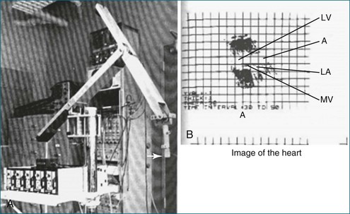
Figure 1-1 A, The mechanical arm used by Dekker and colleagues¹ for tracking the ultrasound transducer in space. Note the arrow depicting the actual ultrasound transducer. As might be imagined, this apparatus was not well received by sonographers because moving the transducer around was physically taxing, given the weight and awkwardness of the mechanical arm. B, Image of the heart. Note that the image shows only mild resemblance to the actual heart and heart chambers. A, aorta; LA, left atrium; LV, left ventricle; MV, mitral valve.

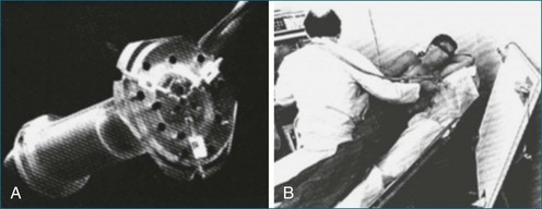
Figure 1-2 An acoustic “spark gap” apparatus used by Moritz and Shreve² for locating the transducer for three-dimensional echocardiography. A, Actual device housing the transducer, with the audio signal sent from the trifurcating mechanism. B, The device in practice, with the coordinates shown on the board to the right of the user.

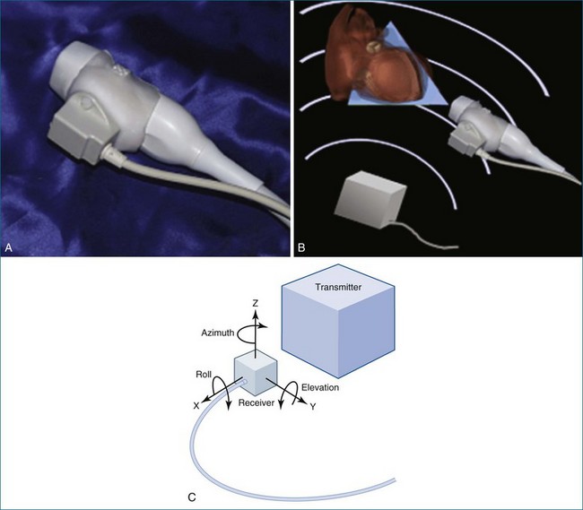
In 1977, Raab and colleagues¹¹ developed the magnetic locator, which ultimately led to the most advanced type of free-hand scanning, but this method for transducer location never caught on until the mid-1990s. This method is still used today by some labs, predominantly for research purposes (Figure 1-3; see also Figures 1-13, 1-14).

Figure 1-3 A, Electromagnetic locator device. The sensor is shown attached to a holder for the transducer. B, Summary of the electromagnetic sensor system. The magnet is located in the box, which serves as the transmitter. The magnet is connected to the sensor and indirectly to the ultrasound system. C, The location of the transducer is tracked by the electromagnetic sensor.

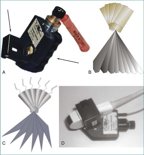
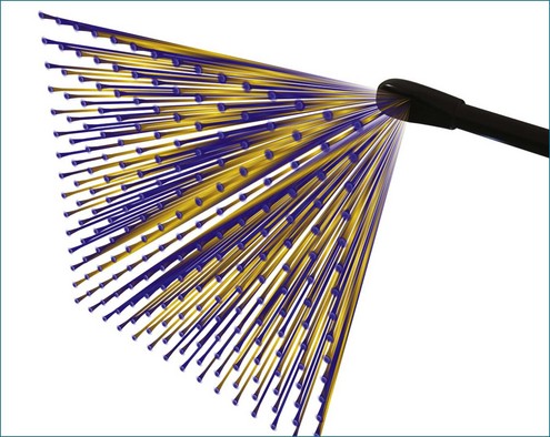
In between the spark gap and the free-hand magnetic approaches were myriad tactics that used the technique of transducer movement in a preprogrammed, stepwise fashion while attempting to keep the patient and the sonographer as stationary as possible. The mechanical devices then moved the transducer in a linear, fanlike, or rotational direction. An example of a fanlike acquisition is shown in Figure 1-4.

Figure 1-4 A, A fanlike device for three-dimensional acquisition. This device, made by TomTec, Inc., stepped the transducer through a fanlike motion. The transducer was held by the square apparatus (arrows), and the user held the device in a manner similar to a pistol grip. B, The stepwise approach to fanlike scanning. C, Ultrasound transducer being held by the fanlike mechanical device in the direction of acquisition. D, Mechanical fan device and transducer within.

(B, Courtesy TomTec, Inc., Munich, Germany.)

Rotational Scanning

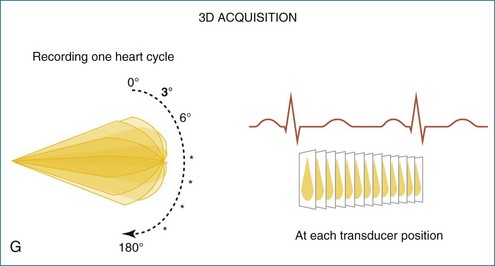
The rotational approach used a cylinder-like mechanical apparatus that those in the industry at that time referred to as the “bazooka” (Figure 1-5). This device had a mechanical stepper motor that moved the transducer sequentially through a semicircular or 180-degree scan with stops every two to three degrees to acquire a 2D image. The acquisition of roughly 60 images was followed by computer software processing, initially using a polar coordinate approach to meld the images into a 3D image. The computer software used significant interpolation between images. The result was frequent “stitch” artifact caused by deficiencies in image line-up from patient movement, transducer movement outside the prespecified position, respiratory or cardiac gating artifact, or all of these factors. Although innovative and potentially very powerful for this era, clear limitations remained. Hence, clinical applicability was very limited.¹³

Figure 1-5 A, A device for rotational scanning with a detachable part for holding different-sized transducers of this era. B, The detachable transducer holder is back in place. C, A transducer (an older mechanical transducer) is shown held in place. D, The rotational device with the attached hardware for connecting to the computer that operated the motor on the rotation stepper. E, Another version of the rotation device produced by TomTec, Inc. F, Rotational scanner shown in close-up. The arrow shows the transducer.G, How rotational scanning was performed with one cardiac cycle obtained every 3 degrees and each cardiac cycle consisting of 15 to 20 frames.

(D and G, Courtesy TomTec, Inc., Munich, Germany.)

Linear or Parallel Scanning

In linear scanning, the transducer was sequentially stepped along a line and obtained images every few millimeters, as opposed to degrees with the rotational and fanlike scans (Figures 1-6 to 1-9). Examples of linear scanning using an intravascular ultrasound, predominantly for coronary imaging, as well as a transthoracic echocardiography (TTE) device are shown in the figures. A device, known as “lobster tail,” for linear pullback using transesophageal echocardiography (TEE) was available as well. In similar fashion as the previously described linear devices, the lobster tail operated by stepwise pullback of the TEE probe in the esophagus, with imaging at each stop. This TEE probe, developed by TomTec, Inc. (Munich, Germany), included both the TEE probe and the “stepper,” that is, the device that moved the probe sequentially (see Figures 1-8 and 1-9). There were several iterations of this technique, including one that involved placing the TEE probe in a water bath within the esophagus to serve as a “standoff” to improve acoustic effects and sharpen the images (see Figure 1-8). The rotational method of scanning with the lobster tail is summarized in Figure 1-9. Further summaries regarding the various types of scanning, early fetal ultrasound, and early computer hardware are shown in Figures 1-10 to 1-12.

Figure 1-6 Parallel, or linear, scanning. In this schematic, the transducer is sequentially “stepped” through the heart following a linear motion.

Figure 1-7 Parallel, or linear, scanning. In these iterations of three-dimensional scanning, the transducer was moved in a linear, stepwise fashion. A and B, The linear stepper device for use with an intravascular ultrasound device. C, A linear stepper for a transthoracic transducer.

(Courtesy TomTec, Inc., Munich, Germany.)

Figure 1-8 A, Linear scanning using the “lobster tail” device for transesophageal echocardiographic (TEE) imaging. B, Details of the TEE probe and how it slides within a carriage. C, A water-filled standoff, or offset, used to improve image quality with TEE imaging.

(B and C, Courtesy TomTec, Inc., Munich, Germany.)

Figure 1-9 Summary of acquisition and processing of three-dimensional data using the linear approach with the “lobster tail” transesophageal echocardiography system. A, Acquisition hardware acquires one full cardiac cycle (14 to 20 frames) at every transducer position and then processes the information into a cube, or volume, of data. B and C, The hardware.

(Courtesy TomTec, Inc., Munich, Germany.) ECG, electrocardiographic.

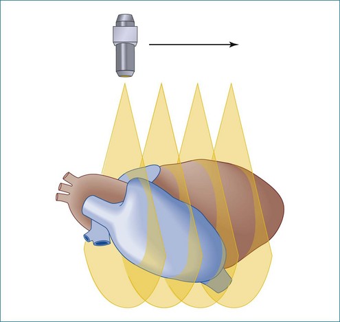
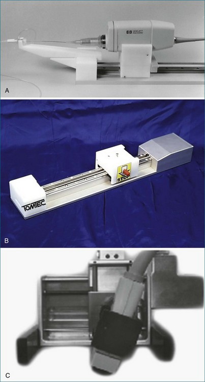
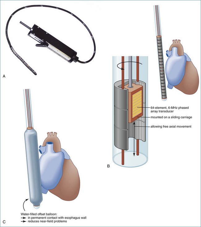
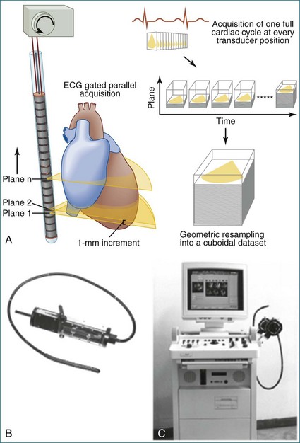
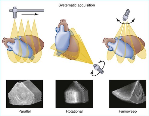
Figure 1-10 Summary of linear (parallel), rotational, and fanlike scanning.

(Courtesy TomTec, Inc., Munich, Germany.)

Figure 1-11 A and D, The Compact 3D Review, an early review station for three-dimensional echocardiography processing. B, C, and E, Early review stations and image acquisition hardware. The Echo-Scan was a computer workstation and image acquisition device combined. The Echo-Scan could be attached to a standard B-mode ultrasound system and its transducer to acquire two-dimensional images in the preprogrammed approach (linear, fanlike, or rotational).

(Courtesy TomTec, Inc., Munich, Germany.)

Figure 1-12 Early fetal images performed using standard B-mode ultrasound and the TomTec Echo-Scan system.

(Courtesy TomTec, Inc., Munich, Germany.)

More Advanced Free-Hand Scanning

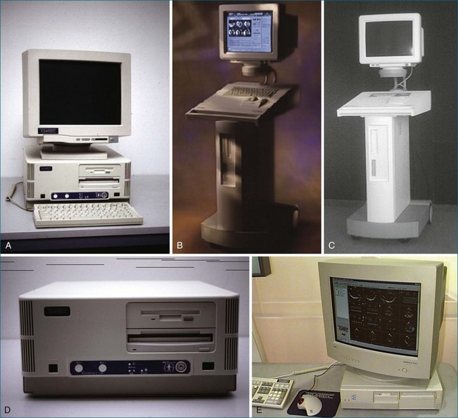
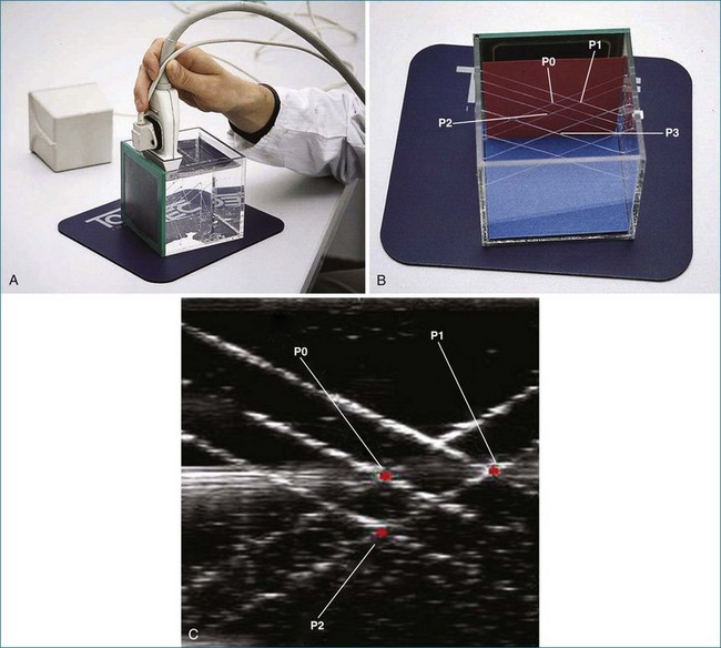
Later, using the technology developed by Raab, free-hand scanning became commercially available from TomTec and from 3D Echo Tech (Boulder, CO; later acquired by GE Medical systems). Both systems used an enhanced version of the electromagnetic detector described by Raab in 1977 (Figures 1-13 and 1-14; see also Figure 1-3). A magnet was enclosed in a plastic housing and placed close to the patient. The electromagnetic locator was electrically wired to a sensor that was placed on the ultrasound transducer and connected to a microcomputer and the commercially available ultrasound system. This enhanced version of the electromagnetic detector is still commercially available today through Ascension Technologies (Milton, VT). Before using this device for free-hand scanning, a calibration must be performed, typically using a phantom that had multiple wires passing through a water bath (see Figure 1-14). This process is tedious and time consuming and is a major reason for the lack of clinical acceptance. Currently, companies that use the electromagnetic sensor for free-hand scanning often hire out the calibration process so the user does not need to become involved in the process. An example of quantitative left ventricular imaging using the method the electromagnetic locator is provided by Legget et al.¹⁴ As computing power improved in the late 1980s and early 1990s, the data processing algorithms for 2D images became advanced and allowed direct conversion of basic images from a polar coordinate system to the cartesian coordinate system. With the evolution of interpolation, gaps between images could be filled, and with the addition of smoothing algorithms, the images could be more systematically reconstructed to resemble an entire heart—or at least individual ventricles.

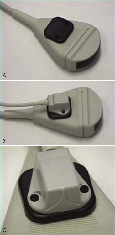
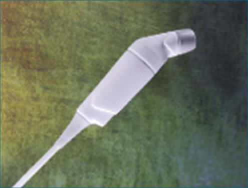
Figure 1-13 A to C, Electromagnetic sensor placed on a general ultrasound transducer.

(Courtesy TomTec, Inc., Munich, Germany.)

Figure 1-14 A, The procedure for performing a calibration of the electromagnetic free-hand scanning apparatus. The transducer is scanning in a water bath; the wires in the bath are set at a known distance and are used as calibration points. B, More details of the wires used for calibration. C, How the wires appear in ultrasound imaging.

(A and C, Courtesy TomTec, Inc., Munich, Germany.)

On-Board Rotational 3D Transesophageal and Transtracheal Echocardiogrphy

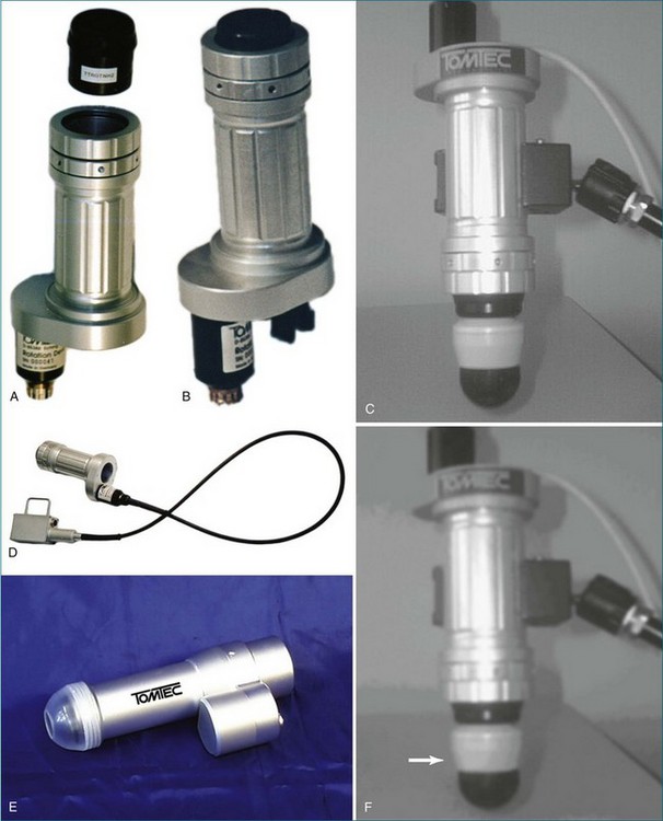
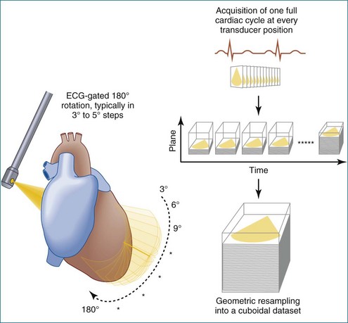
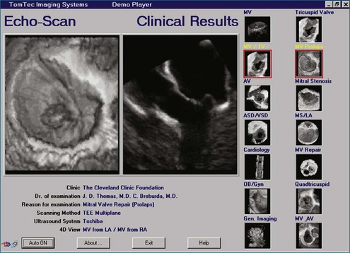
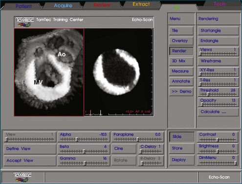
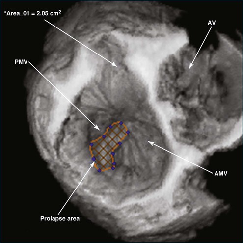
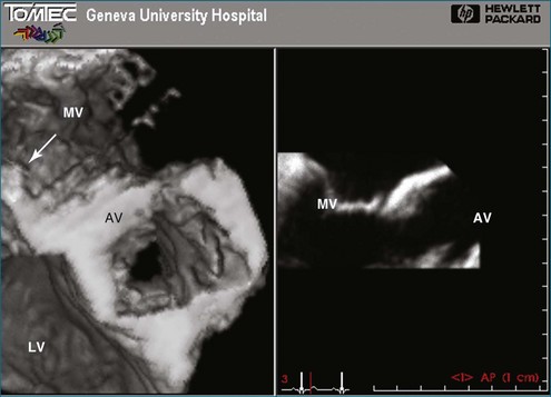
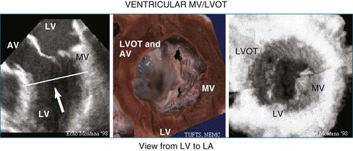
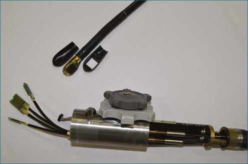
In 1993, TomTec partnered with Hewlett-Packard (HP, Palo Alto, CA) to develop a rotation motor for the existing HP TEE multiple probe (Omniplane I) (Figure 1-15). This allowed rotational scanning using an already available TEE probe. In 1995, the partnership between TomTec and HP progressed even further and led to the development of software that was embedded in the HP 5500 Ultrasound system (Figure 1-16). The technique for this system is summarized in Figure 1-17. Examples of some of the images obtained with the rotational TEE approach are shown in Figures 1-18 to 1-23. In addition, HP developed a transthoracic transducer during the same period (see Figure 1-23). Although a transducer with the rotational mechanism contained within the ultrasound probe was much less cumbersome than holding a conventional probe within the rotational device (shown in Figure 1-5), the image quality was not found to be superior and this transducer was short lived. For the next 7 years or so, 3DE would mostly be performed with the rotational TEE approach. This approach occasionally was quite impressive in the evaluation of the mitral valve but did not offer much for evaluating LV function and size, particularly for quantification.^15,16

Figure 1-15 A, A standard transesophageal echocardiography (TEE) probe (Omniplane I, Hewlett-Packard, Palo Alto, CA) fitted with a stepper motor made by TomTec used to drive the Omniplane TEE through a rotation, with preprogrammed stops at every few angle advancements (typically 3 degrees). B, A grayscale image of a three-dimensional image acquired with the Omniplane TEE and the rotational stepper motor. Note the rotational artifacts (arrows) caused by interpolation of the two-dimensional images between angle stops.

(Courtesy TomTec, Inc., Munich, Germany.)

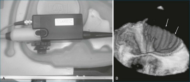
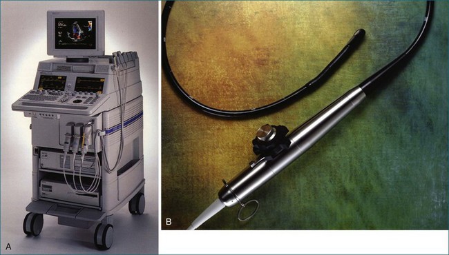
Figure 1-16 Later, Hewlett-Packard and TomTec, Inc. partnered to use a standard ultrasound system (the HP 5500, A) and standard transesophageal echocardiography (TEE) probe (the Omni II, B) and an onboard software program that achieved the same result as shown in Figure 1-15 without needing external hardware to drive the TEE probe.

(Courtesy TomTec, Inc., Munich, Germany.)

Figure 1-17 A summary of how rotational three-dimensional (3D) transesophageal echocardiography was performed. An electrocardiography (ECG)-gated 180-degree rotation was performed with stops every 3 degrees to acquire a two-dimensional (2D) image. The 2D images were collected and, using computer interpolation, contained into a volume of data that could then be rendered into 3D images and cut in multiple planes.

(Courtesy TomTec, Inc., Munich, Germany.)

Figure 1-18 An image acquired from rotational three-dimensional transesophageal echocardiography showing mitral valve prolapse.

(Courtesy TomTec, Inc., Munich, Germany.)

Figure 1-19 An image acquired from rotation three-dimensional transesophageal echocardiography showing the aortic valve (Ao) and mitral valve (MV).

(Courtesy TomTec, Inc., Munich, Germany.)

Figure 1-20 An image of mitral valve prolapse obtained using rotational three-dimensional transesophageal echocardiography imaging. AMV, anterior mitral valve; AV, aortic valve; PMV, posterior mitral valve.

(Courtesy TomTec, Inc., Munich, Germany.)

Figure 1-21 Rotational three-dimensional transesophageal echocardiography imaging showing the aortic valve (AV), left ventricle (LV), and mitral valve (MV).

(Courtesy TomTec, Inc., Munich, Germany.)

Figure 1-22 Mitral valve (MV) prolapse shown from the left ventricular side. The left image shows two-dimensional posterior MV prolapse. The center image shows MV prolapse in a pathologic specimen viewed from the left ventricular side. The right image shows the three-dimensional image of MV prolapse from the ventricular side as well as the left ventricular outflow tract (LVOT). AV, aortic valve; LV, left ventricle.

(Courtesy TomTec, Inc., Munich, Germany.)

Figure 1-23 Rotational transthoracic transducer. A transducer developed by Hewlett Packard used software on board a standard ultrasound system (HP 5500) developed by TomTec, Inc., to rotate the transducer.

(Courtesy Hewlett-Packard, Palo Alto, CA.)

Real-Time Three-dimensional Methods

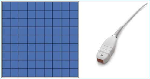
RT3DE was first developed by von Ramm at Duke University during the early 1990s.^17,18 With RT3DE, an entire cardiac volume was obtained in one cardiac cycle. Since only one cardiac cycle was used, there was no “stitch” artifact caused by interpolation between multiple 2D images. The good news was that a volume of data had been acquired. The bad news, however, was that the output was in the form of multiple cross-sectional views of the LV that had the look of parasternal short-axis views. This gave rise to the term C scan (Figure 1-24). Each C scan was a cross-sectional cut through the 3D dataset. Note that in Figure 1-24, A and B, the four- and two-chamber orthogonal views are shown, as well as C1 and C2, the sequential short-axis or axial cuts through the heart. This technology was made commercially available in 1997 by Volumetrics (Chapel Hill, NC) (Figure 1-25). However, the ultrasound system was very large and did not have a separate transducer for performing 2D imaging. Hence, only what was supposedly 3D imaging could be performed. This technology used a sparse-array transducer, as shown in Figure 1-26, with not all of the area of the transducer head being connected to individual elements. In addition, to derive true 3D volume rendering, an offline workstation had to be used. Hence, there were no truly “live” 3D echo images. Volumetrics did show RT3DE rendering at the 2000 American Heart Association meetings, but within months after this showing, the company ceased operations. Undoubtedly, this was a business decision based on the knowledge that a similar, yet much more advanced product was already well into the development stage at HP. The development stage for RT3DE began at HP around 1996. As mentioned earlier, HP had already been a force in the industry when the company co-developed rotational 3D TEE scanning with TomTec and released that product to the general market in 1995. By late 1998, HP had a working prototype for transthoracic RT3DE; it was undoubtedly being tested at specialized 3D centers such as those at the thorax center in Rotterdam, The Netherlands; by Dr. Andreas Francke in Hannover, Germany; and at the University of Chicago echocardiography lab in the United States. HP began showing the prototypes to luminary customers by 1999. A major development in the history of RT3DE came in 1999 when HP spun off its medical division and other computer technology divisions into an entity called Agilent Technologies (Andover, MA). The next year, the medical division of Agilent (excluding the measurement and chemical testing divisions) was bought by Philips Medical Systems of The Netherlands, now known as Philips Health Care. Philips had bought another ultrasound company in 1998, Advanced Technology Laboratories (ATL) of Bothell, Washington, in 1998. Hence, after the HP spinoff to Agilent, the purchase of Agilent by Philips and the already existing ATL, the plan was to merge the ultrasound knowledge to further develop 3D technology as well as other echocardiography applications. The U.S. headquarters for Philips Health was established in Andover, Massachusetts, and the sales headquarters in Bothell, Washington. Thereafter, in 2002, at the time of the American Heart Association meetings, Philips released the first generation of its RT3DE, which used a transthoracic transducer. This transducer, which was significantly larger that standard 2D transducers, was a dense-array transducer (Figures 1-27 to 1-29) and had more than 3000 elements, as opposed to the 256 in the sparse-array unit.

Figure 1-24 Images obtained using the Volumetrics three-dimensional system. The system was originally developed by Duke University and then commercialized by Volumetrics (Chapel Hill, NC).

(Courtesy David Adams, Duke University, Durham, NC.)

Figure 1-25 A, The Volumetrics (Chapel Hill, NC) prototype three-dimensional (3D) imaging system. This prototype developed by Duke University was very large and made exclusively for 3D imaging. It did not have transducers exclusive for two-dimensional imaging. As a result, it was largely purchased by organizations that wanted to perform research studies rather than for clinical use. C, This Model 1 instrument was the first production model by Volumetrics, Inc., circa 1998. B and D-F, The progression of Volumetrics 3D imaging from 1996 to 2000. The company folded shortly after the introduction of the model shown in F.

(Courtesy David Adams, Duke University, Durham, NC.)

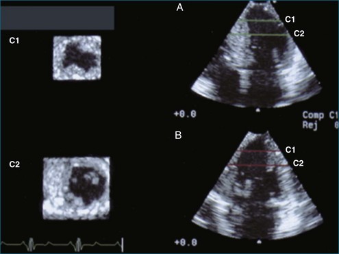
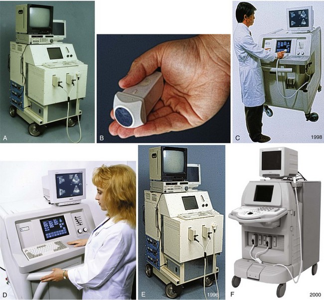
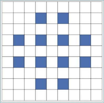
Figure 1-26 The Volumetrics (Chapel Hill, NC) system used sparse-array imaging, which limited image resolution.

Figure 1-27 Dense-array imaging. Real-time three-dimensional imaging, first introduced in 2002 by Philips Medical Systems (now Philips Health Care, Andover, MA) used dense-array imaging.

Figure 1-28 The matrix transducer used for dense-array imaging by Philips Medical Systems (now Philips Health Care, Andover, MA).

Figure 1-29 The first-generation Matrix (Philips Health Care, Andover, MA) transducer (left), second-generation Matrix transducer (middle), and third-generation Matrix transducer, with the latter similar to the standard two-dimensional transducer.

Two years later, at the 2004 American Heart Association meetings, General Electric Health Care (Chalfont St. Giles, United Kingdom) would follow suit with its versions of RT3DE. Similarly, Toshiba introduced RT3DE at the 2007 American College of Cardiology Annual Scientific Sessions in New Orleans, Louisiana. Siemens (Erlangen, Germany) and the U.S. ultrasound group in Issaquah, Washington, would introduce their transthoracic RT3DE system in late 2008. All these RT3DE systems use a transthoracic transducer as well as a matrix-type, dense-array transducer. Because of this approach, the transducer in these products is considerably larger than that used in 2D imaging.

In 2004 and in 2006, Philips Medical Systems released significant upgrades to the 3D systems with the introduction of the ie33 imaging system; General Electric also made major upgrades in 2008 and in 2010, with the introduction of the i9 imaging system.

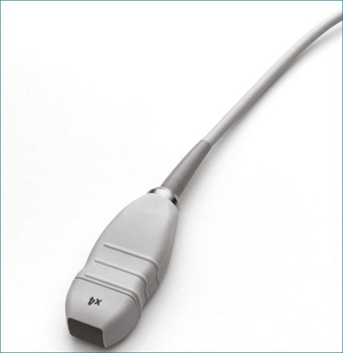
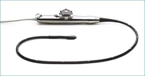
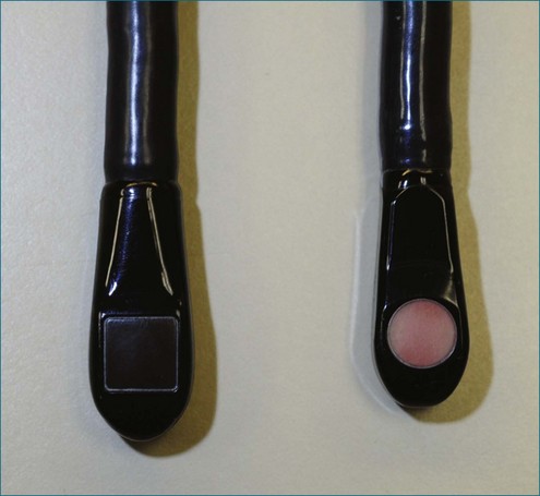
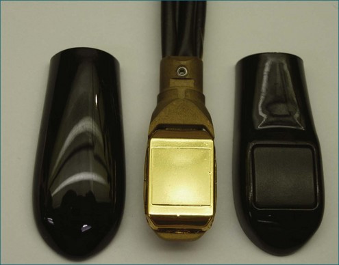
The greatest impact on patient care with regard to 3D and RT3DE happened when Philips introduced the RT3DTEE probe in 2007 at the American Heart Association meetings and earlier that year in Europe (Figures 1-30 to 1-34). At the time of this writing, General Electric is releasing an RT3DTEE system, 5 years after the release of the first one by Philips Health Care. RT3DTEE has been a particular advance with regard to patient treatment, particularly for the treatment of structural heart disease in the interventional lab. Treatments involving percutaneous intervention on the mitral valve are now possible using RT3DTEE guidance. The use of RT3DTEE in the interventional lab is outlined in Chapter 15.

Figure 1-30 The Matrix three-dimensional transesophageal echocardiography probe introduced by Philips Medical Systems (now Philips Health Care, Andover, MA) in 2007.

Figure 1-31 The Matrix transesophageal echocardiography (TEE) probe (left) and the standard Omni III two-dimensional (2D) TEE probe (right) (both Philips Health Care, Andover, MA). Note that control of the Matrix TEE probe is entirely electronic, as opposed to mechanical in the previous 2D echocardiography probe.

Figure 1-32 The Matrix transesophageal echocardiography transducer shown with the external covering front and back (at left and right) and the internal electronic mechanics (center).

Figure 1-33 Steering mechanism for the Matrix three-dimensional transesophageal echocardiography probe (Philips Health Care, Andover, MA).

Figure 1-34 Schematic of how the Matrix three-dimensional transesophageal echocardiography probe (Philips Health Care, Andover, MA) sends out parallel scan lines on the lateral and elevation plane, creating a volume or, more properly, a frustum, of imaging data.

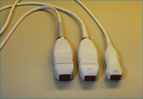
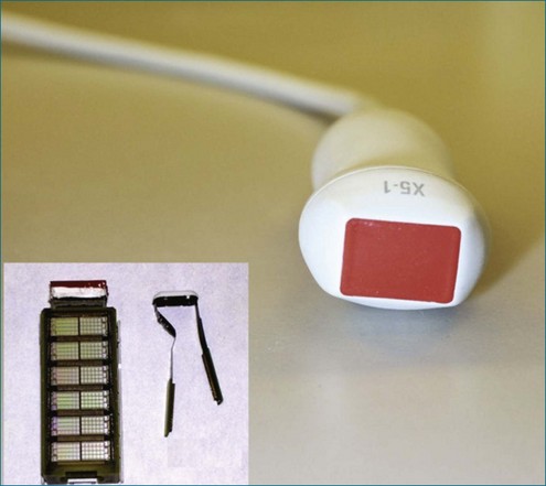
Finally, in 2010, Philips Health Care introduced a TTE transducer for both RT2D and RT3DE imaging (Figure 1-35). The X5 transducer is the world’s first miniaturized matrix-type transducer that allows the user to perform both 2D and 3D echocardiographic imaging without switching transducers, with comparable 2D and 3D image quality.

Figure 1-35 The X5 transducer, the third-generation and latest Matrix transthoracic three-dimensional transducer for transthoracic imaging (Philips Health Care, Andover, MA). It is similar in size and shape to the same-level two-dimensional transducer, the S5.

The development of RT3DE in 2002 by Philips Health Care was a step that made the greatest impact toward 3DE being used on a regular basis by clinical cardiologists and not merely in the research arena. With its 2002 introduction, RT3DE has become more commonplace throughout the United States and worldwide. In fact, 3D technology has proliferated more widely and quickly into Europe and Asia than in United States. Further proliferation continues on a near exponential curve as the technology continues to improve, becomes more miniaturized, and develops more user-friendly interfaces with clearer integration into clinical practice without affecting the general workflow. This fact is discussed in more detail in Chapter 3.

In January 2006, two new 3D ultrasound billing codes were introduced: (1) RT3DE acquisition and analysis, and (2) offline analysis using a separate workstation. How this coding evolves over time will also have an impact on the clinical practice of echocardiography in the years to come.

Since the initial release of RT3DE by Philips in 2002, the volume of data generated from research in the field is enormous, with more than 3000 articles on 3DE cited on Medline during this period. A position paper and summary paper were published by the American Society of Echocardiography in 2007 to guide clinicians in the use of 3DE.^19,20 The European Society of Cardiology has provided a website called 3D Echo Box to guide clinicians through all the articles that describe the use of 3D echocardiography (http://www.escardio.org/communities/EAE/3d-echo-box/Pages/welcome.aspx). The most recent guidelines were published in the January 2012 issue of the Journal of the American Society of Echocardiography.²¹