[level-membership-for-radiology-category]Chapter 2
Haemodynamics and Blood Flow
Principles of Blood Flow
This section describes the simple principles of blood flow which are of value in understanding the role of Doppler and for performing vascular ultrasound examinations. The underlying principles of fluid mechanics applied to the flow of blood are complex, and discussed in detail in a number of texts including those by McDonald,1 Caro et al.,2 Strackee & Westerhof3 and chapters in the Doppler ultrasound books by Evans et al.4 and Taylor et al.5
TYPES OF FLOW
The two essential flow states are laminar and turbulent. At low velocity, fluid flow is laminar (Fig. 2-1A). This is characterised by the motion of fluid along well-defined paths called streamlines. At very high velocities, fluid flow is turbulent (Fig. 2-1B); particular elements of the fluid no longer travel along well-defined paths, and there is a random component to the motion of the fluid.
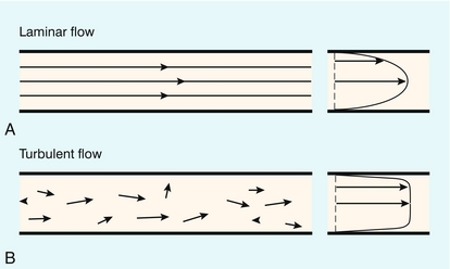
FIGURE 2-1 (A) Laminar flow consists of flow along well-defined streamlines; the velocity profile in a long straight tube under conditions of steady flow is parabolic. (B) The velocity vector magnitude and direction in turbulent flow have random components; the time-averaged profile is blunt.

where ρ is the fluid density, L is the vessel diameter, V is the mean velocity and μ is the fluid viscosity. For a wide variety of fluids the transition to turbulence takes place at a value of Re of about 2000. For flow in which Re is about 2000 the fluid flow will alternate between turbulent and laminar. When velocity is increased so that the Re is above the critical value, turbulence will take a small amount of time to develop. During pulsatile flow it is therefore possible for the flow to be laminar at values of Re higher than the critical value, because turbulence does not have time to develop before the blood velocity has decreased.
The effect of the flow state on the Doppler waveform is illustrated in Figure 2-2. Doppler spectra are shown from the normal femoral artery in Figure 2-2A; in this case flow is laminar. Within the sample volume the blood velocity magnitude and direction are similar for all of the red cells, hence the spectral width is low and the waveform outline is smooth. In the post-stenotic region of a diseased artery the Doppler waveform is more complex (Fig. 2-2B). The blood which was at rest in the poststenotic region during diastole is accelerated through the sample volume. For this blood, flow is laminar and the initial up-slope of the waveform has a smooth outline with low spectral width, whereas blood which was in the prestenotic region during diastole has to pass through the stenosis, producing disturbed and turbulent flow within the sample volume. The variation in velocity magnitude and direction which this produces results in an increase in the spectral width (Fig. 2-2B), and the waveform outline is no longer smooth.
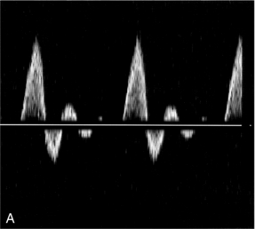

FIGURE 2-2 Femoral artery Doppler waveforms. (A) From a normal segment; the waveform has a smooth outline and the spectral width is low. (B) From the poststenotic region; in the early systolic phase the waveform has a clearly defined outline associated with the passage of blood which was at rest in the poststenotic region during diastole through the insonation site. In the later part of the waveform, blood which has passed through the stenosis has developed turbulent, disturbed flow with increased velocity. This appears as a region in which there is spectral broadening, with Doppler shifts above and below the baseline and high-frequency spikes.
A summary of points concerning flow state is given in Box 2.1.
PRESSURE AND ENERGY
This is a simple expression which dem+onstrates that there will be an interchange between the different types of energy within the circulation. In the human body, however, the flow is not steady and the above equation must be modified slightly to account for the energy required to accelerate the fluid.4 Energy is conserved in this simple ideal lossless system. In the circulation, energy is lost in the form of heat through viscous effects, manifested through friction of the blood at the vessel wall and between adjacent layers of blood. Energy losses are highest in the region of a stenosis, as there is considerable friction during turbulent flow and vortex motion.
The most common application of Bernoulli’s equation is in the prediction of pressure drop across a stenosed cardiac valve.6 The equation may be simplified to:

where V is the measured velocity in m/s, and P is the pressure drop in mmHg. Points concerning pressure and energy are summarised in Box 2.2.
VELOCITY PROFILES
Strictly speaking, a parabolic velocity profile only applies to steady laminar flow in a long straight tube, when there is maximum velocity in the centre of the vessel and zero velocity at the edge of the vessel (Fig. 2-1A). The profile is radially symmetric, which means that it is the same regardless of which diameter is considered. The shape of the profile is an exact mathematical equation, that of a parabola.
Entrance Effect
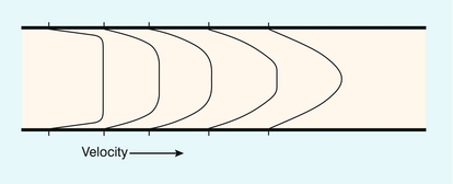
The velocity profile in a vessel is strongly influenced by the distance of the region of interest from the entrance to the vessel. For a long straight vessel, when there is steady flow, the profile is initially flat at the entrance to the vessel. With increasing distance from the entrance the profile will change, becoming parabolic at a distance called the inlet length (Fig. 2-3).
Vessel Narrowing
For steady flow, a gradual narrowing taper will tend to sharpen the velocity profile.
Vessel Expansion
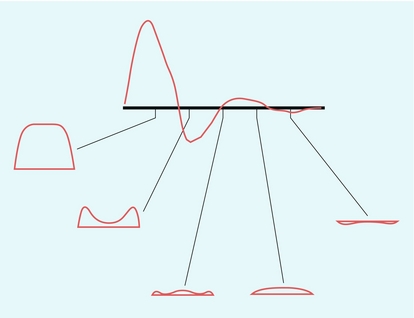
At regions where the cross-sectional area of the vessel increases, an adverse pressure gradient in the direction of flow is created; that is, there is a pressure decrease in the direction of flow, which tends to retard the flow. For the central high-velocity region, the high momentum opposes this, but at the edge of the vessel the velocities are low and the direction of motion near the wall will reverse if there is a sufficiently rapid increase in vessel cross-sectional area with distance. The phrase ‘flow separation’ is often used to describe this phenomenon; that is, the high-velocity central jet is located next to a region in which the flow is of low velocity and recirculating. The production of vortices in these circumstances was noted above; both the central jet and vortices die out after a length equivalent to a few diameters and laminar flow is re-established. Figure 2-4 shows the velocity profiles in the region of a small stenosis. When the expansion is less severe, such as a gradually widening taper, the velocity profile simply becomes more blunted.
Curved Vessels
Figure 2-5 shows that the velocity profile for steady flow in a curved vessel is skewed towards the outer wall when the entrance profile is parabolic, and skewed towards the inner wall when the entrance profile is flat.
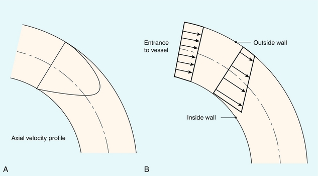
FIGURE 2-5 Velocity profiles within a curved vessel during steady flow. (A) A parabolic velocity profile at the entrance results in higher velocities on the outer aspect of the curve. (B) A blunt velocity profile at the entrance results in the higher velocities occurring on the inner aspect. (From Caro et al.2, with permission.)
Y-Shaped Junction
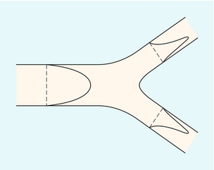
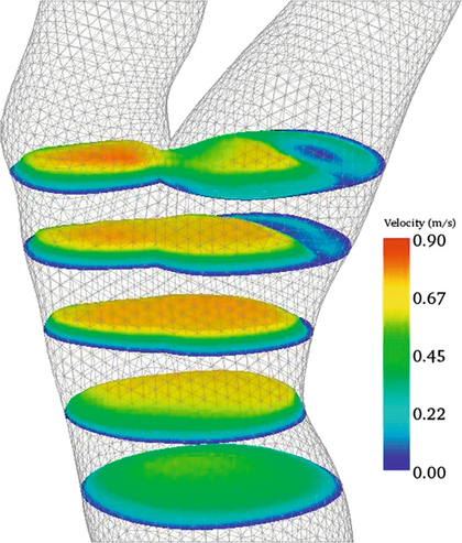
Figure 2-6 shows the velocity profiles from a Y-shaped junction and it can be seen that the profiles are skewed within the two branches, so that the higher velocities occur on the inner aspects of the two branches. Figure 2-7 shows 2D velocity profiles taken in a realistic carotid bifurcation model with a moderate stenosis just proximal to the bifurcation at peak systole. Velocity profiles are reasonably symmetric in the common carotid and in the stenosis, but there is clear asymmetry at the entrance to the internal carotid artery.
Pulsatile Flow
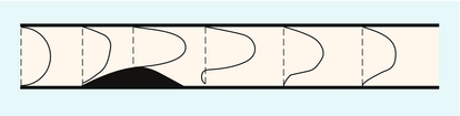
During pulsatile flow the velocity profile will vary throughout the cardiac cycle. Figure 2-8 shows the profiles from a long straight tube with a velocity waveform similar to that found in the femoral artery.
Turbulence
As discussed above, the velocities during turbulence have a random component, so that it is necessary to take an average value over time. If this is done, then the averaged velocity profile during steady turbulent flow is found to be blunted, with high-velocity gradients near to the vessel wall (Fig. 2-1B).
Secondary Flow Motions
In many of the geometrical situations described above the components of flow are three-dimensional, which means that there will be some secondary flow motion in the plane perpendicular to the vessel axis. These motions may easily be demonstrated using flow models and dye-injection techniques, and there are a few in vivo studies which claim to have demonstrated this.7,8
A summary of points concerning velocity profiles is given in Box 2.3.
A SIMPLE FLOW MODEL
where Q is the flow through the vessel, and P1 and P2 are the pressures at the entrance and exit points of the vessel. One way of expressing this equation is to say that in order to maintain flow at a constant level, the pressure difference must be greater when the resistance to flow increases. Strictly speaking this formula only applies for steady flow conditions; it is therefore useful mainly as an aid in understanding general concepts of flow in arteries, and a more complex version of this equation must be used for pulsatile flow. For a long straight vessel the resistance to flow depends on the fourth power of the diameter. A segment of vessel 2 mm in diameter will therefore have a resistance 16 times that of a similar segment of 4 mm diameter.
A simple model of the flow to an organ is shown in Figure 2-9. The net flow is controlled by a combination of the small vessel (arteriolar) resistance and the large vessel (arterial) resistance. In the non-diseased circulation, the main arteries have relatively large diameters and their resistance to flow is small; the main resistance vessels are the arterioles. The essential clinical manifestations of atherosclerosis may be understood with the aid of this model; an increase in resistance in a large distributing artery because of atheroma must be compensated by a decrease in the resistance of the small arteries and arterioles in order to preserve flow to the capillary bed. As the disease progresses, flow is maintained by arteriolar dilatation until the point is reached where the arteriolar network is fully dilated. Further progression of the proximal disease results in a reduction in flow to the organ and the development of ischaemia because no further compensatory dilatation is achievable. In patients with lower limb claudication, the presence of severe proximal disease results in the distal arteriolar network being fully dilated at rest in order to maintain flow to the lower limb muscles. Whilst this is sufficient in the resting limb, the combination of the proximal stenosis and the maximum arteriolar dilatation means that no further increase in flow can be obtained to cope with the increased metabolic demands of limb exercise.
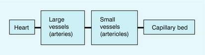
FIGURE 2-9 A simple model of flow from the heart to an organ through a large vessel (arterial) and small vessels (arterioles) to the capillary bed.
The concept of a critical stenosis follows from the above model. As the degree of narrowing at a single, isolated stenosis increases, a point is reached at which the distal arteriolar dilatation is at maximum. Consequently, any increase in the degree of stenosis beyond this point leads to a reduction in flow. Experiments performed on animals suggest that this point of critical stenosis is reached with an area reduction of about 90%, which corresponds to a diameter reduction of approximately 70%. Two quantities of interest in Doppler ultrasound are the volume flow rate and the velocity of the blood; the relationship between these two parameters, according to the model developed above, is shown in Figure 2-10.9 As the calibre of the vessel is reduced, the volume of blood flowing along the vessel is maintained by increasing the velocity. However, above the point of critical stenosis (70% diameter stenosis), the volume of blood starts to reduce. It should also be noted that the velocity peaks at about 85% diameter stenosis, subsequently tailing off, so that in very tight stenoses the velocity is relatively low.
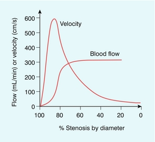
FIGURE 2-10 Flow rate and velocity based upon a single arterial stenosis inserted into an otherwise normal artery. (After Spencer and Reid9, with permission)
The concept of a critical stenosis is useful but its application to atherosclerosis should not be taken too far. As atherosclerosis develops, various other compensatory mechanisms come into play in an attempt to preserve perfusion. These include the development of a collateral circulation and a degree of local dilatation of the affected arterial segment. In addition, there is an increase in the extraction efficiency of oxygen from blood. A summary for this section is given in Box 2.4.
PULSATILE FLOW AND DISTAL RESISTANCE
For a particular element of blood it is the pressure gradient, not the actual pressure, which accelerates the blood. The pressure gradient is related to the difference between the pressures on either side of the element of blood (Fig. 2-11). When the pressure gradient is positive the blood will be accelerated along the vessel; when the gradient is negative the blood will be decelerated. The corresponding flow waveform is found by detailed calculation of the pressure gradient at the site of interest.
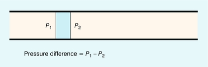
FIGURE 2-11 The force acting on an element of blood is related to the difference in pressures on either side of that element.
Blood ejected by the heart in systole passes into the aorta, where it causes local expansion of the aorta and distal arteries due to the local high pressure. The expanded region passes down the arterial tree in the form of a pressure wave (Fig. 2-12). If the artery were long and straight then, at a particular location along the vessel, the pressure would reach a maximum and then decline to the baseline value (Fig. 2-13A), resulting in a flow waveform with forward flow only (Fig. 2-13B).10 In practice it is known that flow waveforms in arteries can exhibit periods of reverse flow and this section is concerned with understanding the origin of this reverse flow.
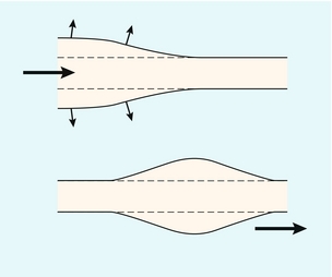
FIGURE 2-12 The blood ejected by the heart causes expansion of the elastic arteries. This expansion passes down the arteries in the form of pressure and flow waves.
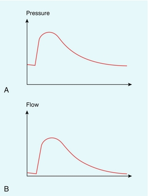
FIGURE 2-13 (A) and (B) Pressure and flow waves in the absence of distal reflection. (From Murgo et al.10, with permission.)
Periods of reverse flow typically occur in arteries which supply muscle at rest, for example the brachial artery or the femoral arteries. However, on exercise, or during periods of reactive hyperaemia, the reverse flow disappears, and there is forward flow throughout the cardiac cycle. This difference in flow waveform is due to differences in the amplitude of reflected pressure and flow waves. As noted above in a long straight pipe there are no reflected waves. However the arterial system is a branching network and the site of the branches will cause a portion of the pressure wave to be reflected and travel back upstream. The major source of reflected waves occurs at the arteriolar junctions, which are the major resistance vessels in the body (Fig. 2-14). When the arterioles are tightly constricted as in the case in resting muscle the amplitude of reflected waves is high, leading to reverse flow. On the other hand, during exercise or reactive hyperaemia the arterioles are dilated, the amplitude of reflected waves is low and the reverse flow component is lost. This relationship between the degree of diastolic flow and the downstream resistance is used as a diagnostic tool, for example in obstetrics where umbilical artery Doppler waveforms are used to provide an indicator of placental resistance to flow. The normal placenta has a low resistance to flow and umbilical waveforms show flow throughout the cardiac cycle. Absent end-diastolic flow is associated with increased resistance to flow and abnormal placental development with an increased incidence of fetal compromise. Studies in sheep have provided good evidence for the basis for this work.11
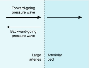
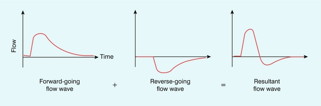
Before considering the detail of how reflected waves give rise to reverse flow, it is worth considering the simple phenomenon of water waves to illustrate some of the concepts. If a buoy is placed in the ocean it will move up and down with the waves, but the height of the buoy does not provide any information on the direction of travel of the wave. If two waves are travelling towards each other from opposite directions and cross each other at the location of the buoy, then the height of the buoy will double as the waves cross due to the additive effect arising from two waves. Returning to the arterial system, there will be a reflected (reverse-going) pressure wave which will travel back up the arterial tree and combine with the forward-going pressure wave in an additive manner, hence the combined pressure will be greater (Fig. 2-15). There is also a reflected (reverse-going) flow wave which will also travel back up the arterial tree. However in the case of the flow wave the direction of motion is important. Because the reverse-going flow wave is travelling in the opposite direction to the forward-going flow wave, the result will be a subtraction of the reverse-going from the forward-going wave, which then results in reverse flow (Fig. 2-16).
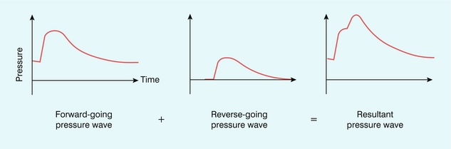
FIGURE 2-15 The resultant pressure wave is a combination of the forward-going wave and the reverse-going wave.
Quantitative Flow Measurement
Whilst it is possible to measure blood flow quantitatively, the error is usually rather large, probably between 20% and 100%.12,13 In some applications such errors may be tolerable, for instance when a large change in flow in the order of 300% from normal to abnormal flow exists. However, one factor which mitigates against blood flow being a sensitive indicator of disease affecting an organ or limb is that circulatory regulatory mechanisms can often maintain the level of blood supply until the disease is quite advanced.
1. Flow is pulsatile, therefore the velocity varies over the cardiac cycle. The velocity also varies across the vessel lumen. In addition, turbulence and disturbed flow will result in vectors of flow off the central axis of the vessel, leading to inaccurate angle estimation and correction. Complex flow patterns can occur in curved vessels and near bifurcations, so that the assumption of laminar or plug flow should be carefully examined for each application. Turbulence observed in a sonogram or colour Doppler image makes accurate measurement of volume flow impossible.
2. In practice it is difficult to ensure uniform insonation of a blood vessel, and the resultant error in instantaneous average velocity can be very large, perhaps greater than 50%. Maximum velocity, for use in the calculation of instantaneous average velocity (see below), can be measured to around 5% by ensuring that the ultrasound beam passes through the centre of the vessel. It should always be borne in mind that spectral broadening errors can be large, up to 50%, when maximum velocity is measured by wide-aperture arrays.14
3. The calibre of compliant arteries varies with the cardiac cycle. Pulsation of an artery can change its cross-section by up to 20%, hence an instantaneous diameter measurement (see below) should be used if possible.
4. The accuracy of the measurement of the vessel diameter, or cross-sectional area, is inversely related to the size of the vessel and measurement errors are usually quite large, up to 20% for a 10 mm diameter vessel, rendering the technique of doubtful value for small vessels. The cross-sectional area and the velocity should be measured at the same site; in addition, errors will occur if the scan plane is not exactly at right angles to the axis of the vessel. Special efforts should be made to reduce the error in diameter measurement, since diameter is squared in the formula for cross-section (area = πr2) and this increases the error.
5. For laminar flow in a straight vessel the beam–vessel angle can be determined to within 2° or 3°. However, even with this accuracy, if the beam–vessel angle is made greater than 60ᵒ, the error in the calculated velocity rapidly rises above 10%, so that the calculated velocities will have significant errors associated with them in this situation.

‘Instantaneous’ means the value measured at the point in the cardiac cycle being considered.
Averaging the instantaneous flow rate over the cardiac cycle gives the average flow rate.

In these cases the time-averaged maximum velocity (TAVmax) can be calculated over several cardiac cycles and, assuming parabolic flow, divided by two to give a calculated time-averaged mean velocity (TAVmean). Some systems will calculate the time-averaged mean velocity directly from the spectral display. Similarly, only a few systems will provide a time-averaged diameter measurement and therefore an instantaneous diameter measurement must be used to calculate area, usually from an image frozen in systole. Alternatively, the area of the vessel can be measured directly from a transverse image of the vessel, providing care is taken to ensure that the section is a true cross-section of the vessel made at systole.
Measurement of volumetric flow is difficult and not generally attempted, as it is easy to produce errors of 100%,12 but there is little in the literature that gives accurate data on errors in practice. In general terms it should be considered as a research tool and the results treated with suitable caution with regard to the potential errors.
Arterial Motion
The degree of arterial distension is related to the elasticity of the artery; stiff arteries will not stretch much, whereas elastic arteries will stretch more. It is possible to estimate an index of elasticity, called pressure strain elastic modulus, from distension and blood pressure.15

This provides an easy estimate of arterial stiffness, allowing applications in patients with, for example, abdominal aortic aneurysm.16 The pressure strain elastic modulus is a measure of the structural stiffness of the artery and is dependent on the thickness of the arterial wall. It would be very desirable to measure the bulk modulus of the artery, also called the Young’s modulus; however this requires knowledge of the wall thickness, which is difficult to measure using ultrasound imaging.
Measurement of wall motion on commercially available systems is slowly being introduced. These are aimed mainly at an assessment of flow-mediated dilatation. This is the phenomenon whereby the mean arterial diameter will increase slightly following a brief period of absent blood flow. Usually the brachial artery is considered and flow is stopped by inflating an arm cuff for a short period of time. The degree of diameter increase following cuff release is used as a measure of endothelial function. Studies over many years have shown that the overall diameter increase may be measured using ultrasound.17,18
REFERENCES
1. McDonald, D. A. Blood flow in arteries. London: Edward Arnold; 1974.
2. Caro, C. G., Pedley, T. J., Schroter, R. C., et al. The mechanics of the circulation. Oxford: Oxford University Press; 1978.
3. Strackee, J., Westerhof, N. The physics of heart and circulation. Bristol: Institute of Physics; 1993.
4. Evans, D. H., McDicken, W. N., Skidmore, R., et al. Doppler ultrasound: physics, instrumentation and clinical applications. Chichester: Wiley; 1989.
5. Taylor, K. J. W., Burns, P. N., Wells, P. N. T. Clinical applications of Doppler ultrasound. New York: Raven Press; 1995.
6. Holen, J., Aaslid, R., Landmark, K., et al. Determination of pressure gradient in mitral stenoses with a non-invasive ultrasound Doppler technique. Acta Med Scand. 1976; 199:455–460.
7. Hoskins, P. R., Fleming, A., Stonebridge, P., et al. Scan-plane vector maps and secondary flow motions. Eur J Ultrasound. 1994; 1:159–169.
8. Stonebridge, P. A., Hoskins, P. R., Allan, P. L., et al. Spiral laminar flow in vivo. Clin Sci. 1996; 91:17–21.
9. Spencer, M. P., Reid, J. M. Quantitation of carotid stenosis with continuous wave (CW) Doppler ultrasound. Stroke. 1979; 10:326–330.
10. Murgo, J. P., Col, M. C., Westerhof, N., et al. Manipulation of ascending aortic pressure and flow waveform reflections with the Valsalva manoeuvre: relationship to input impedance. Circulation. 1981; 63:122–132.
11. Adamson, S. L., Morrow, R. J., Langille, B. L., et al. Site-dependent effects of increases in placental vascular resistance on the umbilical arterial velocity waveform in fetal sheep. Ultrasound Med Biol. 1990; 16:19–27.
12. Evans, D. H. Can ultrasonic duplex scanners really measure volumetric flow? In: Evans J. A., ed. Physics in medical ultrasound. York: Institute of Physical Sciences in Medicine, 1986.
13. Gill, R. W. Measurement of blood flow by ultrasound: accuracy and sources of error. Ultrasound Med Biol. 1985; 11:625–641.
14. Hoskins, P. R. Accuracy of maximum velocity estimates made using Doppler ultrasound systems. Br J Radiol. 1996; 69:172–177.
15. Peterson, L. H., Jensen, R. E., Parnell, J. Mechanical properties of aneurysms in vivo. Circ Res. 1960; 8:622–639.
16. Wilson, K. A., Lee, A. J., Lee, A. J., et al. The relationship between aortic wall distensibility and rupture of infrarenal abdominal aortic aneurysms. J Vasc Surg. 2003; 37:112–117.
17. Celermajer, D. S., Sorensen, K. E., Gooch, V. M., et al. Noninvasive detection of endothelial dysfunction in children and adults at risk of atherosclerosis. Lancet. 1992; 340:1111–1115.
18. Sidhu, J. S., Newey, V. R., Nassiri, D. K., et al. A rapid and reproducible on line automated technique to determine endothelial function. Heart. 2002; 88:289–292.
19. Hammer, S., Jeays, A., MacGillivray, T. J., et al. Acquisition of 3D arterial geometries and integration with computational fluid dynamics. Ultrasound Med Biol. 2009; 35:2069–2083.
[/level-membership-for-radiology-category][not-level-membership-for-radiology-category]Chapter 2
Haemodynamics and Blood Flow
Principles of Blood Flow
This section describes the simple principles of blood flow which are of value in understanding the role of Doppler and for performing vascular ultrasound examinations. The underlying principles of fluid mechanics applied to the flow of blood are complex, and discussed in detail in a number of texts including those by McDonald,1 Caro et al.,2 Strackee & Westerhof3 and chapters in the Doppler ultrasound books by Evans et al.4 and Taylor et al.5
TYPES OF FLOW
The two essential flow states are laminar and turbulent. At low velocity, fluid flow is laminar (Fig. 2-1A). This is characterised by the motion of fluid along well-defined paths called streamlines. At very high velocities, fluid flow is turbulent (Fig. 2-1B); particular elements of the fluid no longer travel along well-defined paths, and there is a random component to the motion of the fluid.
FIGURE 2-1 (A) Laminar flow consists of flow along well-defined streamlines; the velocity profile in a long straight tube under conditions of steady flow is parabolic. (B) The velocity vector magnitude and direction in turbulent flow have random components; the time-averaged profile is blunt.
where ρ is the fluid density, L is the vessel diameter, V is the mean velocity and μ is the fluid viscosity. For a wide variety of fluids the transition to turbulence takes place at a value of Re of about 2000. For flow in which Re is about 2000 the fluid flow will alternate between turbulent and laminar. When velocity is increased so that the Re is above the critical value, turbulence will take a small amount of time to develop. During pulsatile flow it is therefore possible for the flow to be laminar at values of Re higher than the critical value, because turbulence does not have time to develop before the blood velocity has decreased.
The effect of the flow state on the Doppler waveform is illustrated in Figure 2-2. Doppler spectra are shown from the normal femoral artery in Figure 2-2A; in this case flow is laminar. Within the sample volume the blood velocity magnitude and direction are similar for all of the red cells, hence the spectral width is low and the waveform outline is smooth. In the post-stenotic region of a diseased artery the Doppler waveform is more complex (Fig. 2-2B). The blood which was at rest in the poststenotic region during diastole is accelerated through the sample volume. For this blood, flow is laminar and the initial up-slope of the waveform has a smooth outline with low spectral width, whereas blood which was in the prestenotic region during diastole has to pass through the stenosis, producing disturbed and turbulent flow within the sample volume. The variation in velocity magnitude and direction which this produces results in an increase in the spectral width (Fig. 2-2B), and the waveform outline is no longer smooth.
FIGURE 2-2 Femoral artery Doppler waveforms. (A) From a normal segment; the waveform has a smooth outline and the spectral width is low. (B) From the poststenotic region; in the early systolic phase the waveform has a clearly defined outline associated with the passage of blood which was at rest in the poststenotic region during diastole through the insonation site. In the later part of the waveform, blood which has passed through the stenosis has developed turbulent, disturbed flow with increased velocity. This appears as a region in which there is spectral broadening, with Doppler shifts above and below the baseline and high-frequency spikes.
A summary of points concerning flow state is given in Box 2.1.
PRESSURE AND ENERGY
This is a simple expression which dem+onstrates that there will be an interchange between the different types of energy within the circulation. In the human body, however, the flow is not steady and the above equation must be modified slightly to account for the energy required to accelerate the fluid.4 Energy is conserved in this simple ideal lossless system. In the circulation, energy is lost in the form of heat through viscous effects, manifested through friction of the blood at the vessel wall and between adjacent layers of blood. Energy losses are highest in the region of a stenosis, as there is considerable friction during turbulent flow and vortex motion.
The most common application of Bernoulli’s equation is in the prediction of pressure drop across a stenosed cardiac valve.6 The equation may be simplified to:
where V is the measured velocity in m/s, and P is the pressure drop in mmHg. Points concerning pressure and energy are summarised in Box 2.2.
VELOCITY PROFILES
Strictly speaking, a parabolic velocity profile only applies to steady laminar flow in a long straight tube, when there is maximum velocity in the centre of the vessel and zero velocity at the edge of the vessel (Fig. 2-1A). The profile is radially symmetric, which means that it is the same regardless of which diameter is considered. The shape of the profile is an exact mathematical equation, that of a parabola.
Entrance Effect
The velocity profile in a vessel is strongly influenced by the distance of the region of interest from the entrance to the vessel. For a long straight vessel, when there is steady flow, the profile is initially flat at the entrance to the vessel. With increasing distance from the entrance the profile will change, becoming parabolic at a distance called the inlet length (Fig. 2-3).
Vessel Narrowing
For steady flow, a gradual narrowing taper will tend to sharpen the velocity profile.
Vessel Expansion
At regions where the cross-sectional area of the vessel increases, an adverse pressure gradient in the direction of flow is created; that is, there is a pressure decrease in the direction of flow, which tends to retard the flow. For the central high-velocity region, the high momentum opposes this, but at the edge of the vessel the velocities are low and the direction of motion near the wall will reverse if there is a sufficiently rapid increase in vessel cross-sectional area with distance. The phrase ‘flow separation’ is often used to describe this phenomenon; that is, the high-velocity central jet is located next to a region in which the flow is of low velocity and recirculating. The production of vortices in these circumstances was noted above; both the central jet and vortices die out after a length equivalent to a few diameters and laminar flow is re-established. Figure 2-4 shows the velocity profiles in the region of a small stenosis. When the expansion is less severe, such as a gradually widening taper, the velocity profile simply becomes more blunted.
Curved Vessels
Figure 2-5 shows that the velocity profile for steady flow in a curved vessel is skewed towards the outer wall when the entrance profile is parabolic, and skewed towards the inner wall when the entrance profile is flat.
[/not-level-membership-for-radiology-category]
