General Principles of Pharmacology
HOW DO DRUGS ACT?
Action on Receptors
A compound which binds to a receptor and changes intracellular function is termed an agonist. The classic dose–response relationship of an agonist is shown in Figure 1.1. As the concentration of the agonist increases, a maximum effect is reached as the receptors in the system become saturated (Fig. 1.1A). Conventionally, log dose is plotted against effect, resulting in a sigmoid curve which is approximately linear between 20 and 80% of maximum effect (Fig. 1.1B). Three agonists are shown in Figure 1.2. Agonist A produces 100% effect at a lower concentration than agonist B. Therefore, compared with A, agonist B is less potent but has similar efficacy. Drug C is termed a partial agonist as the maximum effect is less than that of A or B. Buprenorphine is a partial agonist (at the μ-opioid receptor), as are some of the β-blockers with intrinsic activity, e.g. oxprenolol, pindolol, acebutalol, celiprolol.
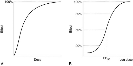
FIGURE 1.1 (A) The effect of an agonist peaks when all the receptors are occupied. (B) A semilog plot produces a sigmoid curve which is linear between 20 and 80% effect. ED50 is the dose which produces 50% of maximum effect.
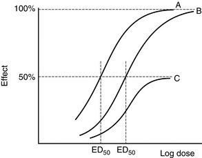
FIGURE 1.2 Agonist B has a similar dose–response curve to A but is displaced to the right. A is more potent than B (smaller ED50) but has the same efficacy. C is a partial agonist which is less potent than A and B and less efficacious (maximum effect 50% of A and B).
Antagonists combine selectively with the receptor but produce no effect. They may interact with the receptor in a competitive (reversible) or non-competitive (irreversible) fashion. In the presence of a competitive antagonist, the dose–response curve of an agonist is shifted to the right but the maximum effect remains unaltered (Fig. 1.3A). Examples of this effect include the displacement of morphine by naloxone and endogenous catecholamines by β-blockers.
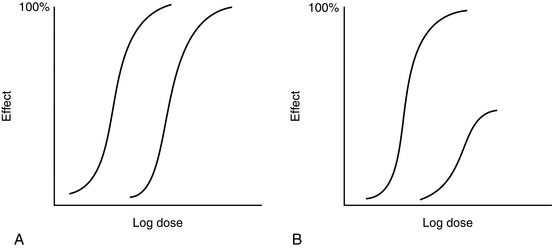
FIGURE 1.3 (A) The dose–response curve of an agonist is displaced to the right in the presence of a reversible antagonist. There is no change in maximum effect but the ED50 is increased. (B) The dose–response curve is displaced to the right also in the presence of an irreversible antagonist but the maximum effect is reduced.
A non-competitive (irreversible) antagonist also shifts the dose–response curve to the right but, with increasing concentrations, reduces the maximum effect (Fig. 1.3B). For example, the α1-antagonist phenoxybenzamine, used in the preoperative preparation of patients with phaeochromocytoma, has a long duration of action because of the formation of stable chemical bonds between drug and receptor.
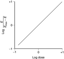
The relationship between drug dose and response is often described by a Hill plot (Fig. 1.4). A typical agonist such as that shown in Figure 1.1 produces a straight line with a slope (i.e. Hill coefficient) of + 1.
THE BLOOD–BRAIN BARRIER AND PLACENTA
The chemoreceptor trigger zone is situated in the area postrema near the base of the fourth ventricle (see Ch 42). It is not protected by the blood–brain barrier because the capillary endothelial cells are not bound tightly in this area and allow relatively free passage of large molecules. This is an important afferent limb of the vomiting reflex and stimulation of this area by toxins or drugs in the blood or cerebrospinal fluid often leads to vomiting. Many antiemetics act at this site.
The transfer of drugs across the placenta is of considerable importance in obstetric anaesthesia (see Ch 35). In general, all drugs which affect the CNS cross the placenta and affect the fetus. Highly ionized drugs (e.g. muscle relaxants) pass across less readily.
METABOLISM
Most drugs are lipid-soluble and many are metabolized in the liver into more ionized compounds which are inactive pharmacologically and excreted by the kidneys. However, metabolites may be active (Table 1.1). The liver is not the only site of metabolism. For example, succinylcholine and mivacurium are metabolized by plasma cholinesterase, esmolol by erythrocyte esterases, remifentanil by tissue esterases and, in part, dopamine by the kidney and prilocaine by the lungs.
TABLE 1.1
Examples of Active Metabolites
| Drug | Metabolite | Action |
| Morphine | Morphine-6-glucuronide | Potent opioid agonist |
| Diamorphine | 6-Monoacetylmorphine Morphine | Opioid agonist |
| Meperidine (pethidine) | Normeperidine (norpethidine) | Epileptogenic |
| Codeine | Morphine | Opioid agonist |
| Diazepam | Desmethyldiazepam Temazepam Oxazepam |
Sedative |
| Tramadol | O-desmethyltramadol | Opioid agonist |
| Parecoxib | Valdecoxib | COX-2 specific inhibitor |
PHARMACOKINETIC PRINCIPLES
Volume of Distribution

where C0 is the initial concentration. Therefore:

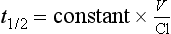
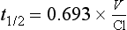
Finally, V can give some indication as to the half-life. A large V is often associated with a relatively slow decline in plasma concentration; this relationship is expressed below in a useful pharmacokinetic equation (eqn 4).
Elimination Half-Life

or
Half-life often reflects duration of action but not if the drug acts irreversibly (e.g. some NSAIDs, omeprazole, phenoxybenzamine) or if active metabolites are formed (Table 1.1).
Calculating t1/2, V and Clearance
It is a simple exercise to calculate these values for a drug after intravenous bolus administration. A known dose is given and regular blood samples are taken for plasma concentration measurements. In this example, we assume that the drug remains in the plasma and is removed only by metabolism; this is a called a one-compartment model. After achieving C0, plasma concentration (CP) declines in a simple exponential manner as shown in Figure 1.5A. If the natural logs of the concentrations are plotted against time (semilog plot), a straight line is produced (Figure 1.5B). The gradient of this line is the elimination rate constant k, which is related to t1/2 in the following equation:
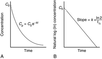
FIGURE 1.5 (A) Exponential decline in plasma drug concentration (CP) in a one-compartment model. The equation predicts CP at any time (t). (B) Semilog plot enables easy calculation of t1/2. Extrapolation of this line enables C0 and AUC∞ to be derived easily.

We may calculate V using equation (2) and then clearance from equation (4). CP may be predicted at any time from the following equation:
where t is the time after administration.

Two-Compartment Models
Let us consider a two-compartment model; one compartment may be thought of as representing the plasma and the other, the remainder of the body. When an intravenous bolus is injected into this system, CP decreases because of an exponential decay resulting from elimination and another exponential decay resulting from redistribution into the tissues. Therefore, when CP is plotted against time, the curve may be described by a biexponential equation. If plotted on a semilogarithmic plot (Fig. 1.6), two straight lines can be identified and derived. Their gradients are the elimination rate constants dependent on elimination (β) and redistribution (α).
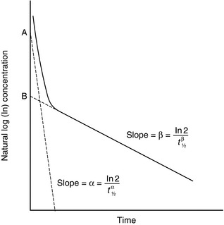
FIGURE 1.6 Semilog plot of a two-compartment model: α = rate constant for exponential decay resulting from redistribution; β = rate constant for exponential decay resulting from elimination.
Calculating the separate pharmacokinetic values is easy; one curve is simply subtracted from the other. Consider Figure 1.6 in which natural log concentration is plotted against time and two slopes are seen. The second and less steep slope represents decline in plasma concentration caused by elimination of the drug by metabolism. From this, the elimination half-life (t1/2β) may be calculated. In order to calculate the half-life of the redistribution phase (t1/2α), the elimination slope is extrapolated back to time 0. If data on this imaginary part of the elimination slope are subtracted from those on the real line above it, another imaginary line may be constructed which represents that part of the decline in plasma concentration which is the result of redistribution. From this line, the redistribution half-life (t1/2α) may be calculated.
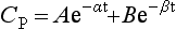
where α and β are the redistribution and elimination rate constants, respectively, and A and B are values derived by back extrapolation of the redistribution and elimination slopes to the y-axis.
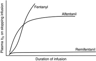
Context-Sensitive Half-Life
Figure 1.7 shows the effect of infusion duration on the half-lives of alfentanil, fentanyl and remifentanil. Alfentanil, and especially fentanyl, accumulate during infusion, causing an increase in context-sensitive half-life as the duration of infusion increases. In other words, time to recovery from alfentanil- or fentanyl-based anaesthesia depends on duration of infusion. Remifentanil is metabolized by tissue esterases and does not accumulate. Therefore, time for plasma concentration of remifentanil to decline by 50% is independent of duration of infusion, i.e. recovery times after remifentanil-based anaesthesia are short and predictable, no matter how long the infusion has run.
PHARMACOGENETICS
The first observations of genetic variation in drug response date from the 1950s, involving the muscle relaxant (succinylcholine [suxamethonium]). Up to 4% of patients have a less efficient variant of the enzyme butyrylcholinesterase (plasma cholinesterase), which metabolizes succinylcholine chloride. As a consequence, the drug’s effect is prolonged to varying degrees (depending on the nature of the abnormal gene and whether the individual is homozygous or heterozygous), with slower recovery from paralysis (see Ch 6).
METHODS OF DRUG ADMINISTRATION
Gastric Emptying
Most drugs are absorbed only when they have left the stomach; therefore, if gastric emptying is delayed, absorption is affected. Furthermore, if oral medication is given continuously during periods of impaired emptying, it may accumulate in the stomach, only to be delivered to the small intestine en masse when gastric function returns, resulting in overdose. Many factors influence the rate of gastric emptying and these are described in Chapter 42.
Intramuscular
Variations in absorption may be clinically relevant. For example, peak plasma concentrations of morphine may occur at any time from 5 to 60 min after intramuscular administration, an important factor in the failure of this method to produce good reliable analgesia (see Ch 41).
Intravenous
Infusion
Drugs may be given by constant-rate infusion, a method used frequently for propofol, neuromuscular blocking agents, opioids and many other drugs. Plasma concentrations achieved during infusions may be described by a simple wash-in exponential curve (Fig. 1.8). The only factor influencing time to reach steady-state concentration is t1/2. Maximum concentration is achieved after approximately 4–5 half-lives. Therefore, this method of administration is best suited to drugs with short half-lives, such as remifentanil, glyceryl trinitrate, Adrenaline and dopamine. However, in practice, it is often used for drugs such as morphine. Assuming a morphine t1/2 of 4 h, it will be about 20 h before steady-state concentration is reached (although an effective concentration can be achieved by initial bolus doses or a more rapid infusion). Therefore, vigilant observation is required with this method of delivery, especially if active metabolites are involved – in this example, morphine-6-glucuronide.
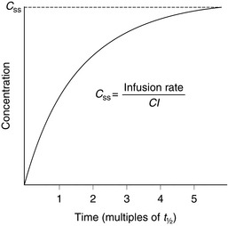
FIGURE 1.8 Plasma concentrations during a constant-rate intravenous infusion against time expressed as multiples of t1/2. Css = concentration at steady state, Cl = clearance.

where Css is the concentration at steady state.
Patient-Controlled Analgesia (PCA)
The use of PCA for the treatment of postoperative pain has become widespread and is described in detail in Chapter 41. The patient titrates opioid delivery to requirements by pressing a button on a PCA device which results in the delivery of a small bolus dose. A lockout time is set which does not allow another bolus to be delivered until the previous dose has had time to have an effect. There is an enormous interpatient variability in opioid requirement after surgery; effective and closely monitored PCA is able to cope with this.
DRUG INTERACTIONS
There are three basic types of drug interaction; examples are listed in Table 1.2.
TABLE 1.2
Examples of Drug Interactions in Anaesthesia
| Type | Drugs | Effect |
| Pharmaceutical | Thiopental: succinylcholine Ampicillin: glucose, lactate Blood: dextrans |
Hydrolysis of succinylcholine Reduced potency
Rouleaux formation |
| Plastic: glyceryl trinitrate Sevoflurane: soda lime | Adsorption to plastic Compound A |
|
| Pharmacokinetic | Opioids: most drugs Warfarin: NSAIDs Barbiturates: warfarin Neostigmine: succinylcholine |
Delayed oral absorption ↑ Free warfarin ↑ Warfarin metabolism ↓ Succinylcholine metabolism |
| Pharmacodynamic | Volatiles: opioids | ↓ MAC |
| Volatiles: benzodiazepines | ↓ MAC | |
| Volatiles: N2O | ↓ MAC | |
| Volatiles: muscle relaxants | ↑ Relaxation | |
| Morphine: naloxone | Reversal (receptor antagonism) | |
| Muscle relaxants: neostigmine | ↑ Relaxation |
VOLATILE ANAESTHETIC AGENTS
The exact mechanism of action of volatile anaesthetic agents is at present unknown. Potency is, in general, related to lipid solubility (Meyer-Overton relationship, Table 1.3) and this has given rise to the concept of volatile agents dissolving in the lipid cell membrane in a non-specific manner, disrupting membrane function and thereby influencing the function of proteins, e.g. ion channels. However, it is now appreciated that volatile agents affect neuronal function as a consequence of binding to specific protein sites (e.g. GABAA receptor).
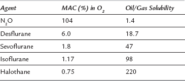
Potency
The potency of volatile agents is defined in terms of minimum alveolar concentration (MAC). MAC is the alveolar concentration of a volatile agent which produces no movement in 50% of spontaneously breathing patients after skin incision. MAC is inversely related to lipid solubility (Table 1.3).
Onset of Action
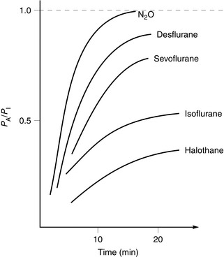
When considering onset of action of volatile agents, there is a fundamental difference compared with intravenous agents. Effects of non-volatile drugs are related to plasma or tissue concentrations; this is not so with volatile agents. Partial pressure of the volatile agent is important, not concentration. If a volatile agent is highly soluble in blood, partial pressure increases slowly because large amounts dissolve in the blood. Consequently, onset of anaesthesia is slow with agents soluble in blood and rapid with agents which are relatively insoluble. The same applies to recovery from anaesthesia. Table 1.4 lists the most commonly used inhaled agents (in order of speed of onset) and their relative blood/gas solubilities.
TABLE 1.4
Solubility of Inhaled Anaesthetic Agents in Blood (Expressed as Blood/Gas Solubility Coefficients)
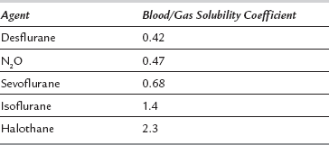
Alveolar partial pressure (PA) is assumed to be equivalent to cerebral artery partial pressure and therefore depth of anaesthesia. At a fixed inspired partial pressure (PI), the rate at which PA approaches PI is related to speed of onset of effect (Fig. 1.9). This is rapid with agents of low blood solubility (e.g. sevoflurane) and relatively slow with more soluble agents (e.g. halothane).