[level-membership-for-critical-care-medicine-category]
169 General Principles of Pharmacokinetics and Pharmacodynamics
Pharmacokinetics and pharmacodynamics describe, respectively, the amount of drug in the body at a given time and the pharmacologic effects caused by the drug.1 Pharmacokinetics describes the movement of a drug into, within, and out of the body over time, whereas pharmacodynamics explains the effects the drug has on the body that result in a clinical response. A general understanding of pharmacokinetic parameters such as clearance, volume of distribution, half-life, steady state, and absorption, along with pharmacodynamic principles such as receptor theory, potency, affinity, tolerance, and minimum effective concentration greatly enhances the clinician’s ability to make informed choices in the treatment of the critically ill patient.
 General Principles of Pharmacokinetics
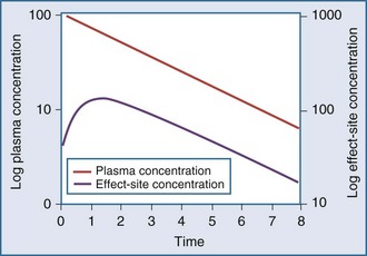
Clearance, volume of distribution, half-life, and bioavailability are four pharmacokinetic parameters that allow the clinician to better estimate dosing requirements. If the concentration of a drug in an easily assessable sampled fluid (e.g., plasma, urine, saliva) correlates well with the pharmacologic response (therapeutic or toxic) to the drug, then the application of pharmacokinetics in dosing is likely to be beneficial.2 Usually the concentration of a drug cannot be measured at the exact site of action (e.g., a receptor on the cell surface), so it is necessary that there be a predictable relationship between the concentration that is measurable and the concentration at the site of the effect.3,4 These concentrations do not have to be equal, but they should reflect a similar direction and magnitude of change over time (Figure 169-1).
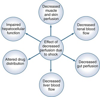
Measurement of the relationship between drug concentration and therapeutic or toxic response in a large number of patients allows development of a therapeutic range or target concentration for that drug (Figure 169-2).5–10 Table 169-1 lists a number of drugs commonly used in the ICU for which therapeutic ranges have been established and for which therapeutic drug monitoring is often recommended.11,12 Critically ill patients have a multitude of host factors (e.g., hemodynamic status, decreased organ function, nutritional status, concurrent disease states) that increase the likelihood that individualized drug dosing based on individualized pharmacokinetic assessment will be beneficial (Figure 169-3).13–16 There can be gender-related differences in both pharmacokinetic and pharmacodynamic responses.17–19 Individual chapters in this text are devoted to many of these agents and their adjustments for dosage in patients with renal or hepatic failure.
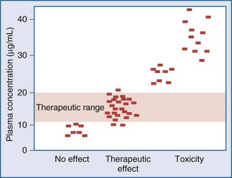
TABLE 169-1 Therapeutic Ranges of Drugs Commonly Used in Critical Care
| Drug | Therapeutic Range |
|---|---|
| Amikacin | Trough < 5 µg/mL |
| Peak < 30 µg/mL | |
| Cyclosporine | Whole blood, 150 ng/mL |
| Digoxin | 0.50-2.0 ng/mL |
| Gentamicin* | Trough < 2 µg/mL |
| Peak < 10 µg/mL | |
| Lidocaine | 1.5-5 µg/mL |
| Phenytoin | 10-20 µg/mL |
| Quinidine | 2-5 µg/mL |
| Theophylline | 10-20 µg/mL |
| Tobramycin* | Trough < 2 µg/mL |
| Peak < 10 µg/mL | |
| Vancomycin† | Trough < 5 µg/mL |
| Peak < 30 µg/mL |
* Once daily aminoglycoside dosing may result in different therapeutic ranges.
† Vancomycin concentrations are currently focusing on higher peak concentrations, and practice varies considerably between sites.
Pharmacokinetic Models
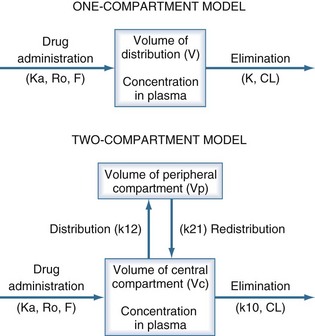
The pharmacokinetic concepts of clearance, volume of distribution, half-life, and bioavailability are based on physiologic principles.20 The physiologic processes governing these concepts are enormously complex, and many simplifying assumptions must be made before the mathematics describing drug concentrations become tractable. Although sophisticated computer modeling approaches are available in research settings, most of the clinically useful pharmacokinetic equations are based on one- or two-compartment models (Figure 169-4).21
Specifically, t1/2 defines the length of time it takes for the drug concentration to decrease by one-half. In a linear pharmacokinetic system with first-order elimination, the t1/2 is a constant, and it takes the same amount of time for the concentration to fall from 100 to 50 arbitrary units as it does to decline from 50 to 25 arbitrary units (Figure 169-5).
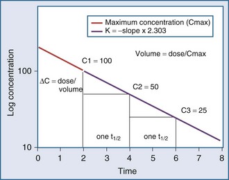
where Δt is the time elapsed between the measurement of two concentrations, C1 and C2. It is the properties of this equation that give rise to the familiar exponentially decreasing concentration-time curve, which becomes linear when plotted on semilog coordinates.
The human body is not a single well-stirred compartment, and it is amazing that such a simple mathematical model can be so useful in the clinical setting. If the body is conceptualized as consisting of individual tissues and organs, the same mathematical treatment can be applied. The concept of the volume of distribution has to be somewhat modified to recognize not only the physical size of the organ or tissue, but also the fact that drugs accumulate to differing degrees in different tissue spaces.22,23 For example, lipophilic drugs have a high affinity for adipose tissue, and this property is reflected by a large partition coefficient (R). The time constant associated with each tissue is a function of the rate of blood flow to that tissue (Q), the physical volume of the tissue (VT), and the partition coefficient. The time constant determines the rate at which equilibrium is reached. As a result, it is possible to construct a set of exponential equations with a time constant unique to each tissue:
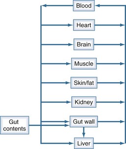
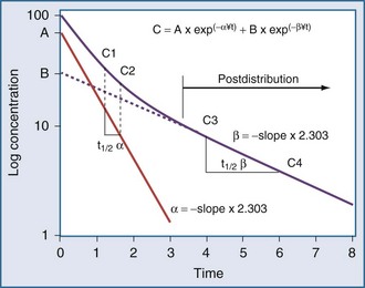
There is a branch of pharmacokinetics known as physiologically based pharmacokinetic modeling that uses blood flows, organ volumes, and partition coefficients to characterize concentration-time profiles.24–27 According to this approach for pharmacokinetic modeling, each tissue space ultimately contributes to the venous pool (Figure 169-6). However, the overall shape of the concentration-time profile in the venous blood is controlled not by the number of tissue spaces or their effective volumes, but by their time constants. Tissues with similar time constants, Q/(V × R), produce similar drug profiles in their venous outflows and appear as a single exponent in pooled venous blood. Practically speaking, many tissues and organs reach equilibrium over similar time frames, and often no more than two distinct time constants are observed. Therefore, this situation can be described adequately by a two-compartment model, characterized by a rapidly distributing central compartment and a more slowly equilibrating peripheral compartment (Figure 169-7). The equation describing the concentration-time profile for the two-compartment model is:
in which β replaces K, can still be used to predict concentrations, as long as both C1 and C2 are in the postdistributive phase. This sum-of-exponentials approach can be extended to three-compartment or even more complex models, but it is difficult to obtain all the concentrations needed to characterize each exponent.
Clearance
Clearance (CL) is a primary pharmacokinetic parameter that measures the ability of the body to eliminate a drug.28,29 It is often stated that clearance is the volume of blood (plasma) that is completely cleared of drug per unit time. Although this is one way to define clearance, it does not capture the relationship between drug clearance (mL/min) and the rate of drug elimination (mg/h). In pharmacokinetics, the general concept of clearance is defined as the rate of elimination relative to the concentration. In a first-order pharmacokinetic system, the rate of elimination is proportional to the drug concentration, and clearance is this proportionality constant:

Clearance is clinically useful because it can be related directly to the organ of elimination. We can talk about renal clearance, hepatic clearance, or biliary clearance, and the sum of each of the individual clearances is the total body clearance.30,31 The immediate clinical consequence is the ability to adjust doses in response to changes in specific organ function. For example, a patient with developing renal failure is likely to require a reduction of the dose of a drug that is eliminated by the kidney, but not necessarily a reduction of the dose of a drug that is eliminated by the liver.32 If the clearance of a drug is known to be 50% renal and 50% hepatic, and renal function is decreased by 50%, it is necessary to reduce the dose by only 25% to maintain the same concentration.

Volume of Distribution
The volume of distribution (V) is another primary pharmacokinetic parameter that is useful in determining the change in drug concentration for a given dose.33 After an intravenous bolus dose in a one-compartment pharmacokinetic model, the change in concentration (ΔC) between Cmax and the concentration immediately before the dose is administered is a function of the dose (D) and the volume of distribution (V):

This equation is useful for predicting both the concentration after a first bolus dose and the increase in concentration at any point in time after a bolus dose. If a concentration before administration of a bolus dose is known or can be estimated, the equation can be used to predict the increase in concentration after the dose is administered (see Figure 169-5). It is important to recognize that the calculated value of ΔC must be added onto the pre-dose concentration to estimate the Cmax after the bolus dose. This equation is also useful for estimating the dose needed to reach a given concentration. If it is known that the volume of distribution is 0.45 L/kg, and a Cmax of 10 mg/L is desired after the loading dose, the dose is estimated to be 10 mg/L × 0.45 L/kg = 4.5 mg/kg. It is not necessary to have a steady-state condition to use this equation, a fact that makes it very useful in critical care.
The volume of distribution increases over time until a distribution equilibrium is reached among all compartments. This is the largest value for the volume of distribution. The fact that distribution equilibrium has occurred can be determined from a log-concentration versus time plot (see Figure 169-7). The curve becomes log-linear when the rate of drug entry into each peripheral compartment equals the rate of exit from each compartment. Because it is often calculated using the clearance and the β or terminal elimination half-life, this volume is often called Vβ:

Half-Life
The half-life (t1/2) is a pharmacokinetic parameter defined as the length of time it takes to reduce the drug concentration by half (see Figure 169-5).33 The half-life is referred to as a secondary parameter because it is a function of the two primary parameters, clearance and volume of distribution:
In a one-compartment system with constant clearance and volume of distribution, drug half-life also is constant. However, in a multicompartment model, the volume of distribution increases over time as drug equilibrates into tissue compartments until Vβ is reached. According to the previous equation, the half-life also increases over time and eventually reaches a maximum at t1/2β (see Figure 169-7).
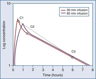
Most drugs have a rapid distribution phase that could be detected if concentrations were measured frequently enough. Aminoglycosides again are a good illustrative example of this concept, because they have a rapid, although not instantaneous, distribution phase (Figure 169-8). With a distribution phase half-life of 5 to 10 minutes, it would take approximately 25 to 50 minutes before the log-linear elimination phase could be observed. It is this distribution process that is the basis for the recommendation to wait approximately 1 hour after the end of an infusion before sampling blood to measure the aminoglycoside concentration. If a blood sample is obtained before this time, the drug still will be in the distribution phase, and the concentration measured will lead to underestimation of the drug half-life. In addition, slowly equilibrating compartments have been demonstrated when aminoglycoside concentrations are measured during washout.34 Aminoglycosides are usually dosed frequently enough so that the slowly equilibrating compartment is not detected.
Bioavailability
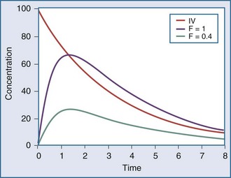
The extent of drug absorption, termed bioavailability (F), is generally referenced to the amount of drug available systemically when the drug is given intravenously. This parameter is determined by comparing the AUC of the drug given by intravenous administration to that of the same drug given by another route (Figure 169-9). The bioavailability of a drug given via the intravenous route is regarded as being 100% (i.e., F = 1.0), and other routes of administration (e.g., oral dosing, intramuscular injection) often have a reduced bioavailability (e.g., F = 0.8, or 80% bioavailability). A number of drug-related and patient-related factors determine bioavailability. In essence, however, F is a function of the degree of absorption and the amount of drug metabolized or eliminated before entering the systemic circulation (first-pass effect).35 Drugs with low bioavailability either cannot be administered by any route other than the intravenous one (e.g., sodium nitroprusside, dobutamine) or require higher doses when given via the oral route compared with the intravenous route (e.g., furosemide, morphine, propranolol). Alternative routes of administration (e.g., rectal, topical, subcutaneous injection, intramuscular injection) are occasionally used in critically ill patients, owing to poor oral bioavailability. These routes all suffer from problems with delayed or poorly predictable serum concentrations. Vasoconstriction, hypoperfusion, edema, gastric suctioning, ileus, diarrhea, and enhanced gastrointestinal motility are all common problems in critically ill patients that can further adversely affect bioavailability.
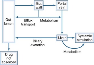
The first-pass effect (Figure 169-10) refers to the elimination of drug that is absorbed orally but then is metabolized by enzymes in the gut wall or in the liver before reaching the systemic circulation. As a drug is absorbed and passes through the gut wall, it can be acted upon by transport proteins (primarily P-glycoprotein) that actively pump drug molecules back into the lumen of the gastrointestinal tract.36–40 All drug molecules that are not pumped out enter the hepatic circulation and are subject to metabolism in the liver before their first opportunity to be presented to the systemic circulation.41 Drugs that have a high hepatic extraction ratio (i.e., are very efficiently removed by the liver) are most likely to show decreased bioavailability due to this first-pass effect; conversely, the bioavailability of these drugs increases if liver dysfunction decreases the hepatic extraction ratio.
Steady State
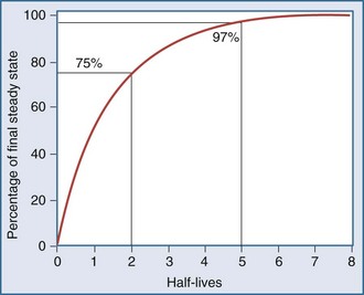
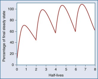
After an infusion is started, drug concentrations increase and eventually reach a concentration that does not change over time (Figure 169-11).42 At this point, the amount of drug entering the body is equal to the amount leaving it during a given period of time, and steady-state conditions apply. During intermittent dosing, drug concentrations accumulate over time, and eventually a steady state is attained. Drug concentrations increase as more drug is administered or absorbed and decrease during elimination, but the concentration profile over each interval resembles all the other profiles during steady state (Figure 169-12). In the clinical setting, measurement of drug concentration is often delayed for a period equal to five half-lives, because at that point the concentration will reflect 97% of the final steady-state concentration.
 Pharmacodynamics
Pharmacodynamics is the study of the relationship between the concentration of a drug and its pharmacologic effect.2 Pharmacodynamic models are routinely employed during drug development, where they are used to determine drug-dosing regimens. These models can become quite complex, particularly if they are mechanism-based models.
Although a pharmacodynamic model can involve many linked mathematical submodels, this is not the type of model that is likely to be useful in a clinical setting. The principles underpinning the relatively simple Emax model are often adequate.43 Mathematically, the equation relating effect and concentration can be described with the Emax equation:
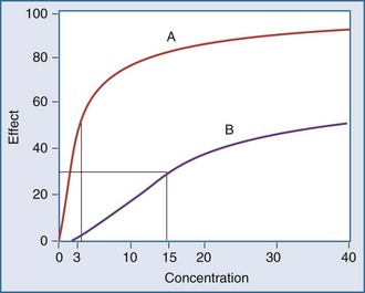
Graphically, this equation has a hyperbolic shape (Figure 169-13). The parameters of this model are the Emax and the EC50. Emax represents the maximal effect attainable due to the drug. The EC50 is the concentration at which half the maximal effect is observed; it is a measure of drug potency. An important feature of this plot reaffirms the intuitive notion that increasing the dose of the drug to higher and higher amounts does not increase the effect of the drug proportionately; eventually, the effect of the drug begins to reach a plateau. In essence, the law of diminishing returns applies: continually smaller increases in effect are observed as the concentration increases. Practically speaking, if the drug concentration is expected to be at the EC50 or lower, increasing the dose will produce a meaningful increase in effect. However, if the concentration exceeds the EC50, increasing the dose may not be warranted, because only small increases in effect may be expected, and the increased concentrations may place the patient at risk for development of adverse (i.e., off-target) drug-related effects.
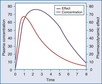
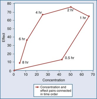
Another point to consider is that time does not appear in the effect model. The concentrations are explicitly defined as steady-state concentrations, and the effect resulting from a given concentration is considered to be a steady-state effect. This model applies when drug in the plasma rapidly equilibrates with drug at the site of action, and there is no indirect mechanism between the concentration at the site of effect and the effect. The more common situation is that the effect lags somewhat behind the concentration (Figure 169-14). If concentrations are going up and coming down over time, as would be expected with an intermittent intravenous or oral dosing schedule, the effect is also expected to go up and down over time, but the time frames may not exactly coincide. For example, the plasma concentration might peak at 1 hour and the effect might peak several hours later. There is a mismatch or disequilibrium between concentration and effect, and a plot of effect versus concentration, with the points connected in time order, yields a hysteresis loop (Figure 169-15). It can be seen that for any given concentration, there are two levels of effect, one on the upswing of the concentration-time curve and the other on the downswing. Both empirical and mechanistic pharmacodynamic modeling approaches have been developed to allow for this disequilibrium. Although the modeling of effect-time curves is achievable, and these models are useful in predicting effects with various dosing regimens, their routine use in clinical settings has been limited.
Protein Binding

Intuitively, it is clear that when a drug is displaced from its binding sites in the plasma, the increase in unbound drug concentration can lead to adverse reactions. A series of scientific papers published in the mid-1960s set this direction for interpretation of the clinical implications of protein binding. In a study of the interaction between warfarin and phenylbutazone, it was shown that phenylbutazone increases plasma warfarin concentration and also increases prothrombin time.44 In addition, warfarin binding was studied in vitro, and it was clearly shown that phenylbutazone displaces warfarin from binding sites. It was concluded that phenylbutazone potentiates the action of warfarin in vivo by displacing warfarin from its binding to plasma albumin, causing more warfarin to be available to specific sites of biological action. Although it may have been intuitive to relate the in vivo and in vitro observations in a cause-and-effect manner, change in protein binding is not the correct explanation for the drug interaction. It is now known that the drug interaction is mediated through an inhibition of the metabolic clearance of warfarin by phenylbutazone.45
The pharmacokinetic concepts concerning the implications of protein binding were reviewed in 2002 by Benet and Hoener.46 The mathematical approach is not repeated here, but when one employs physiologically based models for clearance, volume of distribution, and protein binding, changes in plasma protein binding can be shown to have little clinical relevance. These clearance concepts illustrate that physiologic parameters (intrinsic clearance, organ blood flow, and protein binding) have an impact on some pharmacokinetic parameters, and these changes result in changes to the shape of the plasma-concentration time profiles. However, these effects do not necessarily translate into clinically relevant changes in effective concentrations. To better understand this concept, the relationship between drug exposure and pharmacodynamic effect must be considered.
where fu is the fraction unbound, F is the bioavailability, and CL is the clearance.
To address this issue, Benet and Hoener reviewed pharmacokinetic data on 456 drugs from the literature (Table 169-2). No orally administered drug which has a high elimination ratio and is cleared nonhepatically met the criterion for significant (>70%) protein binding. Only 25 (5%) of the 456 drugs had high extraction ratios, were not administered by the oral route, and met the criterion for which protein binding may influence drug exposure. However, many of these 25 agents are routinely used in critical care (Table 169-3).
TABLE 169-2 Circumstances in Which Changes in Protein Binding Will Affect Unbound AUC
| Low-Extraction-Ratio Drugs | High-Extraction-Ratio Drugs | |
|---|---|---|
| IV Administration | ||
| Hepatic clearance | No | Yes* |
| Nonhepatic clearance | No | Yes* |
| Oral Administration | ||
| Hepatic clearance | No | No |
| Nonhepatic clearance | No | Yes† |
AUC, area under the concentration-time curve; IV, intravenous.
* Only 25 of the 456 drugs reviewed met the criteria.
† None of the 456 drugs reviewed met the criteria.
TABLE 169-3 25 Drugs for Which Changes in Protein Binding May Influence Clinical Drug Exposure After Intravenous or Intramuscular Administration*
| Alfentanil | Itraconazole |
| Amitriptyline | Lidocaine |
| Buprenorphine | Methylprednisolone |
| Chlorpromazine | Midazolam |
| Cocaine | Milrinone |
| Diltiazem | Nicardipine |
| Diphenhydramine | Pentamidine |
| Doxorubicin | Propofol |
| Erythromycin | Propranolol |
| Fentanyl | Remifentanil |
| Gold sodium thiomalate | Sufentanil |
| Haloperidol | Verapamil |
| Idarubicin |
* Criteria for selection included > 70% protein binding and hepatic clearance > 6.0 mL/min/kg or nonhepatic extraction ratio clearance ≥ 0.28 × renal blood flow (>4.8 mL/min/kg).
Modified from Benet LZ, Hoener BA. Changes in plasma protein binding have little clinical relevance. Clin Pharmacol Ther 2002;71:115-21.
In critically ill patients, protein concentrations can change over time. This is particularly true of the acute-phase reactant, α1-acid glycoprotein (AAG). In addition, some patients (e.g., those undergoing dialysis or those with cachexia) have altered protein binding.47,48 Although it might seem intuitive to automatically adjust drug doses in response to changes in protein binding, the information in Table 169-2 should be considered. The extent of protein binding, route of administration, route of elimination, and extraction ratio of the drug all should be considered when determining whether a change in binding is likely to result in a change in effect.49,50
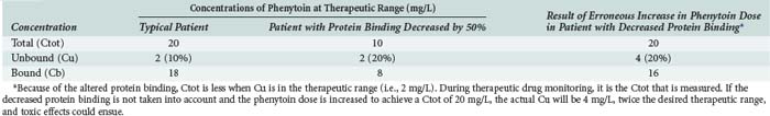
As a final note on protein binding, care must be taken when evaluating drug concentrations in patients with altered protein binding. Consider the case of phenytoin. The percentage of unbound drug is typically 10% but is approximately doubled (to about 20%) in patients receiving hemodialysis (Table 169-4). If phenytoin were administered as a standard dose to all patients, there would not be a problem; phenytoin is a low-clearance drug, and protein binding should not influence overall unbound exposure whether the drug is administered orally or intravenously. However, phenytoin concentrations are often obtained for the purposes of therapeutic drug monitoring, and efforts are made to achieve circulating levels within the commonly accepted therapeutic range of 10 to 20 mg/L. In patients with normal protein binding, this drug level equates to an unbound therapeutic range of 1 to 2 mg/L. However, in patients with a higher percentage of unbound drug, say 20%, the desired unbound concentration is still 1 to 2 mg/L, but the corresponding total concentration is approximately halved. In such cases, if the dose of phenytoin is increased to bring the total concentration into the therapeutic range, toxicities may be observed because the unbound concentration will be approximately twice the desired value.
 Nonlinear Pharmacokinetics
The application of pharmacokinetics to therapeutic drug monitoring becomes considerably more difficult with drugs that exhibit nonlinearities. With linear pharmacokinetics, parameters are stable over time and across concentrations. Doubling of the dose results in doubling of the concentration, and a given dose provides the same AUC regardless of the dosing history, even when the dose in question is the first dose. Nonlinear pharmacokinetics is a term used when the principle of superposition no longer holds. An increase in dose may result in an increase in concentration that is more than or less than proportional, or it may result in clearance changes over time (Figure 169-16). There are several common types of nonlinearities that occur in the clinical setting.51
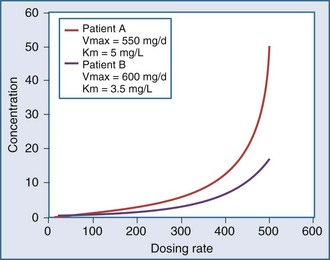
In a linear elimination process, clearance is constant, and doubling the concentration doubles the rate of elimination. In the case of phenytoin with nonlinear elimination, the rate of elimination does not increase in proportion to the concentration, and clearance is not a constant. The nonlinear elimination of phenytoin occurs because the metabolic pathway responsible for the elimination of the drug is saturable. The enzyme system has a maximum rate of metabolism that can be approached at therapeutic concentrations of phenytoin. These principles can be better understood by considering the rate of elimination described by the Michaelis-Menten equation (Figure 169-17). It has two parameters, the maximum rate of elimination (Vmax) and the concentration that results in one-half the maximum rate (Km):
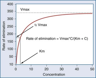
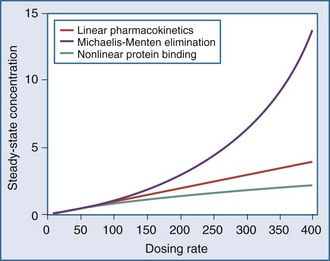
This equation shows that an increase in dosing rate produces a greater than proportional increase in the steady-state concentration. Furthermore, if the dosing rate exceeds Vmax, a steady-state concentration will never be attained. The nonlinear relationship between phenytoin dosing rate and steady-state concentration can be seen for two patients with different Vmax and Km parameters (Figure 169-18). It is easy to understand the difficulties clinicians can encounter when adjusting doses for a drug such as phenytoin which displays nonlinear elimination kinetics. A dose increase that provides a nearly proportional increase in concentration in one patient could produce a much greater concentration in another. These two curves would be straight lines for drugs that displayed linear pharmacokinetics.
Another type of nonlinearity is time-dependent pharmacokinetics. The classic example in this category is the ability of carbamazepine to induce its own metabolism.52 This autoinduction causes the clearance of carbamazepine to increase over time. It is important to gradually increase the dose of carbamazepine during the first few weeks of therapy up to the expected maintenance dose so as to avoid toxicities related to elevated concentrations.

 Alterations in the Elderly
The number of people over 65 years of age is increasing in the United States and in many European countries, and this growth in the elderly population will result in an even greater percentage of ICU beds occupied by older patients. Compared with younger patients, elderly patients typically are taking more drugs, have more underlying organ dysfunction (hepatic, renal, central nervous system), are more likely to be malnourished and to have altered protein binding on this basis, and have reduced or increased responses to some medications.53 These age-related changes further complicate management of the superimposed critical illness because of large variations among individuals with respect to disposition of drugs (Figure 169-19).
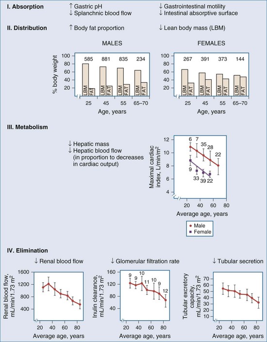
Figure 169-19 Physiologic changes with aging that may affect drug distribution are reflected.
(From Evans WE, Schentag JJ, editors. Applied pharmacokinetics: principles of therapeutic drug monitoring. 3rd ed. Vancouver, WA: Applied Therapeutics; 1992, p. 919-43.)
Elderly patients may have a decreased rate of drug absorption, although the total amount of drug absorbed is usually unchanged. As the body ages, the percentage of body mass that is fat increases. This change results in greater distribution of lipophilic drugs into fat, leading to longer half-lives for certain classes of drugs such as anesthetics, barbiturates, and benzodiazepines. Clearance of many drugs is decreased in the elderly, because the hepatic and renal function decreases with increasing age (Table 169-5). These changes can lead to a greater incidence of toxicity because metabolites associated with adverse effects can accumulate. Overall, the same careful attention to dosing required for all critically ill patients must be extended to the elderly. Drugs should be stopped as soon as possible, and dosage increases should be applied cautiously.
TABLE 169-5 Effects of Aging on Clearance of Some Oxidized and Conjugated Drugs
| Drug | Effect | Reference |
|---|---|---|
| Oxidized | ||
| Chlordiazepoxide | ↓↓ | Am J Psychiatry 1977;134:559 |
| Desmethyldiazepam | ↓↓ | Br J Clin Pharmacol 1979;7:119 |
| Erythromycin | ↓↓ | Eur J Clin Pharmacol 1990;39:161 |
| Haloperidol | ↓↓ | Neuropsychobiology 1996;33:12 |
| Midazolam | ↓↓ | Biochem Pharmacol 1992;44:275 |
| Nicardipine | ↓↓ | Am Heart J 1989;117:256 |
| Nifedipine | ↓↓ | Br J Clin Pharmacol 1988;25:297 |
| Phenytoin (free) | ↓↓ | Clin Pharmacokinet 1981;6:389 |
| Propranolol | — | Br J Clin Pharmacol 1979;7:49 |
| Theophylline | ↓↓ | Eur J Clin Pharmacol 1989;36:29 |
| Verapamil | ↓↓ | Acta Med Scand 1984;681(Suppl):25 |
| Conjugated | ||
| Acetaminophen | ↓ | Br J Clin Pharmacol 1990;30:634 |
| Lamotrigine | ↓ | J Pharm Med 1991;1:121 |
| Lidocaine | ↓↓ | J Cardiovasc Pharmacol 1983;5:1093 |
| Lorazepam | ↓ | Clin Pharmacol Ther 1979;26:103 |
| Metronidazole | — | Hum Exp Toxicol 1990;9:155 |
| Morphine | ↓ | Age Ageing 1989;18:258 |
| Oxazepam | — | Clin Pharmacol Ther 1981;30:805 |
—, no effect; ↓, minor effect; ↓↓, significant effect.
Modified from Woodhouse K, Wynne HA. Age-related changes in hepatic function: implications for drug therapy. Drugs Aging 1992;2:243.
 Pharmacogenomics
It is now recognized that genetic variants exist in drug transporters that influence the distribution of drugs into tissue spaces. Research in this area increased dramatically following the recognition that overexpression of the multidrug-resistance protein, MDR-1, in tumor cells led to a loss of drug effect. This class of efflux proteins functions to pump drugs out of cells and is responsible for reducing drug concentrations in tissues such as the brain, testes, gastrointestinal tract, and biliary tree. There is evidence that the expression of some of these transporters is under genetic control. Concentrations of digoxin reportedly are elevated in patients with low MDR-1 expression.54
Drug effects are often mediated through direct receptor proteins, or proteins that influence control of the cell cycle or signal transduction cascades. Polymorphisms in the expression of these proteins could result in pharmacodynamic differences. For example, a polymorphism has been linked to increased down-regulation of the β2-adrenergic receptor when patients are treated with a β-agonist for amelioration of the symptoms of asthma.55 Genetic polymorphisms leading to altered drug sensitivity also have been identified in angiotensin-converting enzyme, the angiotensin II T1 receptor, and the sulfonylurea receptor.56
Key Points
Benet LZ, Hoener B. Changes in plasma protein binding have little clinical relevance. Clin Pharmacol Ther. 2002;71:115-121.
De Paepe P, Belpaire FM, Buylaert WA. Pharmacokinetic and pharmacodynamic considerations when treating patients with sepsis and septic shock. Clin Pharmacokinet. 2002;41:1135-1151.
Gibaldi M, Perrier D. Pharmacokinetics, 2nd ed. New York: Marcel Dekker; 1982.
Renton KW. Alteration of drug biotransformation and elimination during infection and inflammation. Pharmacol Ther. 2001;92:147-163.
Schulz M, Schmoldt A. Therapeutic and toxic blood concentrations of more than 800 drugs and other xenobiotics. Pharmazie. 2003;58:447-474.
1 Ensom MHH, Davis GA, Cropp CD, Ensom RJ. Clinical pharmacokinetics in the 21st century. Clin Pharmacokinet. 1998;34:265-279.
2 Holford NHG, Sheiner LB. Understanding the dose-effect relationship: Clinical application of pharmacokinetic-pharmacodynamic models. Clin Pharmacokinet. 1981;6:429-453.
3 Meineke I, Freudenthaler S, Hofmann U, et al. Pharmacokinetic modelling of morphine, morphine-3-glucuronide and morphine-6-glucuronide in plasma and cerebrospinal fluid of neurosurgical patients after short-term infusion of morphine. Br J Clin Pharmacol. 2002;54:592-603.
4 de Lange EC, Danhof M. Considerations in the use of cerebrospinal fluid pharmacokinetics to predict brain target concentrations in the clinical setting: Implications of the barriers between blood and brain. Clin Pharmacokinet. 2002;41:691-703.
5 Jenne JW, Wyze MS, Rood FS, et al. Pharmacokinetics of theophylline: Application to the adjustment of the clinical dose of aminophylline. Clin Pharmacol Ther. 1972;13:349-360.
6 Hendeles L, Bighley L, Richardson RH, et al. Frequent toxicity from IV aminophylline infusions in critically ill patients. Drug In tell Clin Pharm. 1977;11:12-18.
7 Jenne JW. Reassessing the therapeutic range for theophylline: Another perspective. Pharmacotherapy. 1993;13:595-597.
8 Weinberger MM, Hendeles L. Reassessing the therapeutic range for theophylline: Another perspective. Pharmacotherapy. 1993;13:598-601.
9 Beauchamp D, Labrecque G. Aminoglycoside nephrotoxicity: Do time and frequency of administration matter? Curr Opin Crit Care. 2001;7:401-408.
10 Begg EJ, Barclay ML, Kirkpatrick CM. The therapeutic monitoring of antimicrobial agents. Br J Clin Pharmacol. 2001;52(Suppl 1):35S-43S.
11 Bauer LA. Clinical pharmacokinetics and pharmacodynamics. In Dipiro JT, Talbert RL, Yee GC, et al, editors: Pharmacotherapy: A Pathophysiologic Approach, 5th ed, New York: McGraw-Hill, 2002.
12 Schulz M, Schmoldt A. Therapeutic and toxic blood concentrations of more than 800 drugs and other xenobiotics. Pharmazie. 2003;58:447-474.
13 De Paepe P, Belpaire FM, Buylaert WA. Pharmacokinetic and pharmacodynamic considerations when treating patients with sepsis and septic shock. Clin Pharmacokinet. 2002;41:1135-1151.
14 Dreisbach AW, Lertora JJ. The effect of chronic renal failure on hepatic drug metabolism and drug disposition. Semin Dial. 2003;16:45-50.
15 Pichette V, Leblond FA. Drug metabolism in chronic renal failure. Curr Drug Metab. 2003;4:91-103.
16 Renton KW. Alteration of drug biotransformation and elimination during infection and inflammation. Pharmacol Ther. 2001;92:147-163.
17 Cummins CL, Wu CY, Benet LZ. Sex-related differences in the clearance of cytochrome P450 3A4 substrates may be caused by P-glycoprotein. Clin Pharmacol Ther. 2002;72:474-489.
18 Schwartz JB. The influence of sex on pharmacokinetics. Clin Pharmacokinet. 2003;42:107-121.
19 Morris ME, Lee HJ, Predko LM. Gender differences in the membrane transport of endogenous and exogenous compounds. Pharmacol Rev. 2003;55:229-240.
20 Tozer TN. Concepts basic to pharmacokinetics. Pharmacol Ther. 1981;12:109-131.
21 Tod MM, Padoin C, Petitjean O. Individualising aminoglycoside dosage regimens after therapeutic drug monitoring: Simple or complex pharmacokinetic methods? Clin Pharmacokinet. 2001;40:803-814.
22 Yokogawa K, Ishizaki J, Ohkuma S, Miyamoto K. Influence of lipophilicity and lysosomal accumulation on tissue distribution kinetics of basic drugs: A physiologically based pharmacokinetic model. Methods Find Exp Clin Pharmacol. 2002;24:81-93.
23 Bjorkman S. Prediction of the volume of distribution of a drug: Which tissue-plasma partition coefficients are needed? J Pharm Pharmacol. 2002;54:1237-1245.
24 Bjorkman S, Wada DR, Berling BM, Benoni G. Prediction of the disposition of midazolam in surgical patients by a physiologically based pharmacokinetic model. J Pharm Sci. 2001;90:1226-1241.
25 Leahy DE. Progress in simulation modeling for pharmacokinetics. Curr Top Med Chem. 2003;3:1257-1268.
26 Curtis CG, Chien B, Bar-Or D, Ramu K. Organ perfusion and mass spectrometry: A timely merger for drug development. Curr Top Med Chem. 2002;2:77-86.
27 Grass GM, Sinko PJ. Physiologically-based pharmacokinetic simulation modelling. Adv Drug Del Rev. 2002;54:433-451.
28 Rowland M, Benet LZ, Graham GC. Clearance concepts in pharmacokinetics. J Pharmacokinet Pharmacodynam. 1973;1:123-136.
29 Sirianni GL, Pang KS. Organ clearance concepts: New perspectives on old principles. J Pharmacokinet Pharmacodynam. 1997;25:449-470.
30 Perri D, Ito S, Rowsell V, Shear NH. The kidney—the body’s playground for drugs: An overview of renal drug handling with selected clinical correlates. Can J Clin Pharmacol. 2003;10:17-23.
31 Patel J, Mitra AK. Strategies to overcome simultaneous P-glycoprotein mediated efflux and CYP3A4 mediated metabolism of drugs. Pharmacogenomics. 2001;2:401-415.
32 Launay-Vacher V, Izzedine H, Mercadal L, Deray G. Clinical review: Use of vancomycin in haemodialysis patients. Crit Care (Lond). 2002;6:313-316.
33 Gibaldi M, Koup JR. Pharmacokinetic concepts: Drug binding, apparent volume of distribution and clearance. Eur J Clin Pharmacol. 1981;20:299-305.
34 Schentag JJ, Jusko WJ, Plaut ME, et al. Tissue persistence of gentamicin in man. JAMA. 1977;238:327-329.
35 Martinez MN, Amidon GL. A mechanistic approach to understanding the factors affecting drug absorption: A review of fundamentals. J Clin Pharmacol. 2002;42:620-643.
36 Lin JH, Yamazaki M. Role of P-glycoprotein in pharmacokinetics: Clinical implications. Clin Pharmacokinet. 2003;42:59-98.
37 Dantzig AH, de Alwis DP, Burgess M. Considerations in the design and development of transport inhibitors as adjuncts to drug therapy. Adv Drug Del Rev. 2003;55:133-150.
38 Faber KN, Muller M, Jansen PL. Drug transport proteins in the liver. Adv Drug Del Rev. 2003;55:107-124.
39 Schinkel AH, Jonker JW. Mammalian drug efflux transporters of the ATP binding cassette (ABC) family: An overview. Adv Drug Del Rev. 2003;55:3-29.
40 Johnson WW. P-glycoprotein-mediated efflux as a major factor in the variance of absorption and distribution of drugs: Modulation of chemotherapy resistance. Methods Find Exp Clin Pharmacol. 2002;24:501-514.
41 Roberts MS, Magnusson BM, Burczynski FJ, Weiss M. Enterohepatic circulation: Physiological, pharmacokinetic and clinical implications. Clin Pharmacokinet. 2002;41:751-790.
42 Wagner JG, Northam JI, Always CD, Carpenter OS. Blood levels of drug at equilibrium state after multiple dosing. Nature. 1965;18:1301-1302.
43 Holford NHG, Sheiner LB. Pharmacokinetic and pharmacodynamic modeling in vivo. Crit Rev Bioengineering. 1981;July:273-322.
44 Aggeler PM, O’Reilly RA, Leong L, Kowitz PE. Potentiation of anticoagulant effect of warfarin by phenylbutazone. New Engl J Med. 1967;276:496-501.
45 Banfield C, O’Reilly RA, Chan E, Rowland M. Phenylbutazone-warfarin interaction in man: Further stereochemical and metabolic considerations. Br J Clin Pharmacol. 1983;16:669-675.
46 Benet LZ, Hoener BA. Changes in plasma protein binding have little clinical relevance. Clin Pharmacol Ther. 2002;71:115-121.
47 Piafsky KM, Borga O, Odar-Cederloff L, et al. Increased plasma protein binding of propranolol and chlorpromazine mediated by disease-induced elevations of plasma alpha-1 acid glycoprotein. N Engl J Med. 1978;299:1435-1439.
48 Mann HJ, Townsend RJ, Fuhs DW, Cerra FB. Decreased hepatic clearance of clindamycin in critically ill patients with sepsis. Clin Pharm. 1987;6:154-159.
49 Bergogne-Berezin E. Clinical role of protein binding of quinolones. Clin Pharmacokinet. 2002;41:741-750.
50 Sparreboom A, Nooter K, Loos WJ, Verweij J. The (ir)relevance of plasma protein binding of anticancer drugs. Neth J Med. 2001;59:196-207.
51 van Rossum JM, van Lingen G, Burgers JPT. Dose-dependent pharmacokinetics. Pharmacol Ther. 1983;21:77-99.
52 Bertilsson L, Tomson T, Tybrig G. Pharmacokinetics: Time-dependent changes—autoinduction of carbamazepine epoxidation. J Clin Pharmacol. 1986;26:459-462.
53 Beyth RJ, Shorr RI. Principles of drug therapy in older patients: Rational drug prescribing. Clin Geriatr Med. 2002;18:577-592.
54 Verstuyft C, Schwab M, Schaeffeler E, et al. Digoxin pharmacokinetics and MDR1 genetic polymorphisms. Eur J Clin Pharmacol. 2003;58:809-812.
55 Silverman ES, Liggett SB, Gelfand EW, Rosenwasser LJ, Baron RM, Bolk S, et al. The pharmacogenetics of asthma: a candidate gene approach. Pharmacogenomics J. 2001;1:27-37.
56 Meisel C, Gerloff T, Kirchheiner J, Mrozikiewicz PM, Niewinski P, Brockmoller J, et al. Implications of pharmacogenetics for individualizing drug treatment and for study design. J Mol Med. 2003;81:154-167.
[/level-membership-for-critical-care-medicine-category][not-level-membership-for-critical-care-medicine-category]
169 General Principles of Pharmacokinetics and Pharmacodynamics
Pharmacokinetics and pharmacodynamics describe, respectively, the amount of drug in the body at a given time and the pharmacologic effects caused by the drug.1 Pharmacokinetics describes the movement of a drug into, within, and out of the body over time, whereas pharmacodynamics explains the effects the drug has on the body that result in a clinical response. A general understanding of pharmacokinetic parameters such as clearance, volume of distribution, half-life, steady state, and absorption, along with pharmacodynamic principles such as receptor theory, potency, affinity, tolerance, and minimum effective concentration greatly enhances the clinician’s ability to make informed choices in the treatment of the critically ill patient.
General Principles of Pharmacokinetics
Clearance, volume of distribution, half-life, and bioavailability are four pharmacokinetic parameters that allow the clinician to better estimate dosing requirements. If the concentration of a drug in an easily assessable sampled fluid (e.g., plasma, urine, saliva) correlates well with the pharmacologic response (therapeutic or toxic) to the drug, then the application of pharmacokinetics in dosing is likely to be beneficial.2 Usually the concentration of a drug cannot be measured at the exact site of action (e.g., a receptor on the cell surface), so it is necessary that there be a predictable relationship between the concentration that is measurable and the concentration at the site of the effect.3,4 These concentrations do not have to be equal, but they should reflect a similar direction and magnitude of change over time (Figure 169-1).
Measurement of the relationship between drug concentration and therapeutic or toxic response in a large number of patients allows development of a therapeutic range or target concentration for that drug (Figure 169-2).5–10 Table 169-1 lists a number of drugs commonly used in the ICU for which therapeutic ranges have been established and for which therapeutic drug monitoring is often recommended.11,12 Critically ill patients have a multitude of host factors (e.g., hemodynamic status, decreased organ function, nutritional status, concurrent disease states) that increase the likelihood that individualized drug dosing based on individualized pharmacokinetic assessment will be beneficial (Figure 169-3).13–16 There can be gender-related differences in both pharmacokinetic and pharmacodynamic responses.17–19 Individual chapters in this text are devoted to many of these agents and their adjustments for dosage in patients with renal or hepatic failure.
TABLE 169-1 Therapeutic Ranges of Drugs Commonly Used in Critical Care
| Drug | Therapeutic Range |
|---|---|
| Amikacin | Trough < 5 µg/mL |
| Peak < 30 µg/mL | |
| Cyclosporine | Whole blood, 150 ng/mL |
| Digoxin | 0.50-2.0 ng/mL |
| Gentamicin* | Trough < 2 µg/mL |
| Peak < 10 µg/mL | |
| Lidocaine | 1.5-5 µg/mL |
| Phenytoin | 10-20 µg/mL |
| Quinidine | 2-5 µg/mL |
| Theophylline | 10-20 µg/mL |
| Tobramycin* | Trough < 2 µg/mL |
| Peak < 10 µg/mL | |
| Vancomycin† | Trough < 5 µg/mL |
| Peak < 30 µg/mL |
* Once daily aminoglycoside dosing may result in different therapeutic ranges.
† Vancomycin concentrations are currently focusing on higher peak concentrations, and practice varies considerably between sites.
Pharmacokinetic Models
The pharmacokinetic concepts of clearance, volume of distribution, half-life, and bioavailability are based on physiologic principles.20 The physiologic processes governing these concepts are enormously complex, and many simplifying assumptions must be made before the mathematics describing drug concentrations become tractable. Although sophisticated computer modeling approaches are available in research settings, most of the clinically useful pharmacokinetic equations are based on one- or two-compartment models (Figure 169-4).21
Specifically, t1/2 defines the length of time it takes for the drug concentration to decrease by one-half. In a linear pharmacokinetic system with first-order elimination, the t1/2 is a constant, and it takes the same amount of time for the concentration to fall from 100 to 50 arbitrary units as it does to decline from 50 to 25 arbitrary units (Figure 169-5).
where Δt is the time elapsed between the measurement of two concentrations, C1 and C2. It is the properties of this equation that give rise to the familiar exponentially decreasing concentration-time curve, which becomes linear when plotted on semilog coordinates.
The human body is not a single well-stirred compartment, and it is amazing that such a simple mathematical model can be so useful in the clinical setting. If the body is conceptualized as consisting of individual tissues and organs, the same mathematical treatment can be applied. The concept of the volume of distribution has to be somewhat modified to recognize not only the physical size of the organ or tissue, but also the fact that drugs accumulate to differing degrees in different tissue spaces.22,23 For example, lipophilic drugs have a high affinity for adipose tissue, and this property is reflected by a large partition coefficient (R). The time constant associated with each tissue is a function of the rate of blood flow to that tissue (Q), the physical volume of the tissue (VT), and the partition coefficient. The time constant determines the rate at which equilibrium is reached. As a result, it is possible to construct a set of exponential equations with a time constant unique to each tissue:
There is a branch of pharmacokinetics known as physiologically based pharmacokinetic modeling that uses blood flows, organ volumes, and partition coefficients to characterize concentration-time profiles.24–27 According to this approach for pharmacokinetic modeling, each tissue space ultimately contributes to the venous pool (Figure 169-6). However, the overall shape of the concentration-time profile in the venous blood is controlled not by the number of tissue spaces or their effective volumes, but by their time constants. Tissues with similar time constants, Q/(V × R), produce similar drug profiles in their venous outflows and appear as a single exponent in pooled venous blood. Practically speaking, many tissues and organs reach equilibrium over similar time frames, and often no more than two distinct time constants are observed. Therefore, this situation can be described adequately by a two-compartment model, characterized by a rapidly distributing central compartment and a more slowly equilibrating peripheral compartment (Figure 169-7). The equation describing the concentration-time profile for the two-compartment model is:
in which β replaces K, can still be used to predict concentrations, as long as both C1 and C2 are in the postdistributive phase. This sum-of-exponentials approach can be extended to three-compartment or even more complex models, but it is difficult to obtain all the concentrations needed to characterize each exponent.
Clearance
Clearance (CL) is a primary pharmacokinetic parameter that measures the ability of the body to eliminate a drug.28,29 It is often stated that clearance is the volume of blood (plasma) that is completely cleared of drug per unit time. Although this is one way to define clearance, it does not capture the relationship between drug clearance (mL/min) and the rate of drug elimination (mg/h). In pharmacokinetics, the general concept of clearance is defined as the rate of elimination relative to the concentration. In a first-order pharmacokinetic system, the rate of elimination is proportional to the drug concentration, and clearance is this proportionality constant:
Clearance is clinically useful because it can be related directly to the organ of elimination. We can talk about renal clearance, hepatic clearance, or biliary clearance, and the sum of each of the individual clearances is the total body clearance.30,31 The immediate clinical consequence is the ability to adjust doses in response to changes in specific organ function. For example, a patient with developing renal failure is likely to require a reduction of the dose of a drug that is eliminated by the kidney, but not necessarily a reduction of the dose of a drug that is eliminated by the liver.32 If the clearance of a drug is known to be 50% renal and 50% hepatic, and renal function is decreased by 50%, it is necessary to reduce the dose by only 25% to maintain the same concentration.
Volume of Distribution
The volume of distribution (V) is another primary pharmacokinetic parameter that is useful in determining the change in drug concentration for a given dose.33 After an intravenous bolus dose in a one-compartment pharmacokinetic model, the change in concentration (ΔC) between Cmax and the concentration immediately before the dose is administered is a function of the dose (D) and the volume of distribution (V):
This equation is useful for predicting both the concentration after a first bolus dose and the increase in concentration at any point in time after a bolus dose. If a concentration before administration of a bolus dose is known or can be estimated, the equation can be used to predict the increase in concentration after the dose is administered (see Figure 169-5). It is important to recognize that the calculated value of ΔC must be added onto the pre-dose concentration to estimate the Cmax after the bolus dose. This equation is also useful for estimating the dose needed to reach a given concentration. If it is known that the volume of distribution is 0.45 L/kg, and a Cmax of 10 mg/L is desired after the loading dose, the dose is estimated to be 10 mg/L × 0.45 L/kg = 4.5 mg/kg. It is not necessary to have a steady-state condition to use this equation, a fact that makes it very useful in critical care.
The volume of distribution increases over time until a distribution equilibrium is reached among all compartments. This is the largest value for the volume of distribution. The fact that distribution equilibrium has occurred can be determined from a log-concentration versus time plot (see Figure 169-7). The curve becomes log-linear when the rate of drug entry into each peripheral compartment equals the rate of exit from each compartment. Because it is often calculated using the clearance and the β or terminal elimination half-life, this volume is often called Vβ:
Half-Life
The half-life (t1/2) is a pharmacokinetic parameter defined as the length of time it takes to reduce the drug concentration by half (see Figure 169-5).33 The half-life is referred to as a secondary parameter because it is a function of the two primary parameters, clearance and volume of distribution:
In a one-compartment system with constant clearance and volume of distribution, drug half-life also is constant. However, in a multicompartment model, the volume of distribution increases over time as drug equilibrates into tissue compartments until Vβ is reached. According to the previous equation, the half-life also increases over time and eventually reaches a maximum at t1/2β (see Figure 169-7).
Most drugs have a rapid distribution phase that could be detected if concentrations were measured frequently enough. Aminoglycosides again are a good illustrative example of this concept, because they have a rapid, although not instantaneous, distribution phase (Figure 169-8). With a distribution phase half-life of 5 to 10 minutes, it would take approximately 25 to 50 minutes before the log-linear elimination phase could be observed. It is this distribution process that is the basis for the recommendation to wait approximately 1 hour after the end of an infusion before sampling blood to measure the aminoglycoside concentration. If a blood sample is obtained before this time, the drug still will be in the distribution phase, and the concentration measured will lead to underestimation of the drug half-life. In addition, slowly equilibrating compartments have been demonstrated when aminoglycoside concentrations are measured during washout.34 Aminoglycosides are usually dosed frequently enough so that the slowly equilibrating compartment is not detected.
