[level-membership-for-surgery-category]Chapter 1
Epidemiology and Clinical Analysis
Louis L. Nguyen, Ann DeBord Smith
The goal of this chapter is to introduce the vascular surgeon to the principles that underlie the design, conduct, and interpretation of clinical research. Disease-specific outcomes otherwise detailed in subsequent chapters will not be covered here. Rather, this chapter discusses the historical context, current methodology, and future developments in epidemiology, clinical research, and outcomes analysis. This chapter serves as a foundation for clinicians to better interpret clinical results and as a guide for researchers to further expand clinical analysis.
Epidemiology
Epidemiology is derived from the Greek terms for “upon” (epi), “the people” (demos), and “study” (logos), and can be translated into “the study of what is upon the people.” It exists to answer the four major questions of medicine: diagnosis, etiology, treatment, and prognosis.
Brief History
Hippocrates is considered to be among the earliest recorded epidemiologists because he treated disease as both a group event and an individual occurrence. His greatest contribution to epidemiology was the linkage of external factors (climate, diet, and living conditions) with explanations for disease. Before widespread adoption of the scientific method, early physicians inferred disease causality through careful observation. For example, they observed the geographic distribution of cases or common factors shared by diseased versus healthy persons. John Snow is recognized for ameliorating the cholera epidemic in the Soho district of London in 1854 by identifying the cause of the outbreak through mapping the location of known cases of cholera in the district. Based on the density and geographic distribution of cases, he concluded that the public water pump was the source and had the pump handle removed.1
Modern Developments
Modern epidemiology and clinical analysis seek to establish causation through study design and statistical analysis. Carefully designed studies and analyses can minimize the risk of false conclusions and maximize the opportunity to find causation when it is present. In other areas of biology, causation can be demonstrated by fulfilling criteria, such as Koch’s postulates for establishing the relationship between microbe and disease. In epidemiology, the study design that would offer ideal proof of causation would be comparison of people with themselves in both the exposed and the unexposed state. This impossible and unethical experiment would control for everything, except the exposure, and thus, establish the causality between exposure and disease. Because this condition cannot exist, it is referred to as counterfactual. Because the ideal study is impossible to conduct, alternative study designs have developed with different risks and benefits. The crossover experimental design, for example, approaches the counterfactual ideal by exposing patients to both treatment groups in sequence. However, the influence of time and previous exposure to the other treatment assignment may still affect the outcome (also known as the carryover effect). Other study designs exist that include techniques such as randomization or prospective data gathering to minimize bias. Appropriate study design must be selected based upon a study’s objectives. After a study is complete, conclusions can be drawn from a carefully crafted statistical analysis. Modern epidemiology includes applied mathematical methods to quantify observations and draw inferences about their relationships.
Evidence-based medicine is a relatively modern approach to the practice of medicine that aims to qualify and encourage the use of currently available clinical evidence to support a particular treatment paradigm. This practice encourages the integration of an individual practitioner’s clinical expertise with the best currently available recommendations from clinical research studies.2 Relying on personal experience alone could lead to biased decisions, whereas relying solely on results from clinical research studies could lead to inflexible policies. Evidence-based medicine stratifies the strength of the evidence from clinical research studies based on study design and statistical findings (Table 1-1). The criteria differ when the evidence is sufficient to support a specific therapeutic approach, prognosis, diagnosis, or other health services research. Criteria also differ among research institutions, including the U.S. Preventive Services Task Force and the U.K. National Health Service. However, common themes can be seen among the different fields. Systematic reviews with homogeneity are preferred over single reports, whereas randomized controlled trials (RCTs) are preferred over cohort and case-control studies. Even within similar study design groupings, the statistical strength of each study is evaluated, with preference for studies with large numbers, complete and thorough follow-up, and results with small confidence intervals. Clinical recommendations are then based on the available evidence and are further graded according to their strengths (Table 1-2).
Table 1-1
Levels of Evidence for Therapeutics
| Level | Evidence |
| 1a | Systematic reviews of RCT studies with homogeneity |
| 1b | Individual RCT with narrow confidence intervals |
| 1c | “All or none” trials* |
| 2a | Systematic reviews of cohort studies with homogeneity |
| 2b | Individual cohort studies |
| 2c | Clinical outcomes studies |
| 3a | Systemic reviews of case-control studies with homogeneity |
| 3b | Individual case-control studies |
| 4 | Case-series studies |
| 5 | Expert opinion without critical appraisal or based on bench research |
* In which all patients died before the therapeutic became available, but some now survive with it, or in which some patients survived before the therapeutic became available, but now none die with it.
RCT, Randomized controlled trial.
Adapted from Oxford Centre for Evidence-based Medicine (2001).
Table 1-2
Grades of Recommendation
| Grade | Recommendation | Basis |
| A | Strong evidence to support practice | Consistent level 1 studies |
| B | Fair evidence to support practice | Consistent level 2 or 3 studies or extrapolations from level 1 studies |
| C | Evidence too close to make a general recommendation | Level 4 studies or extrapolation from level 2 or 3 studies |
| D | Evidence insufficient or conflicting to make a general recommendation | Level 5 evidence or inconsistent studies of any level |
Adapted from U.S. Preventive Services Task Force Ratings (2003) and Oxford Centre for Evidence-based Medicine (2001).
Clinical Research Methods
Although measuring the incidence and prevalence of disease is useful in the initial understanding of a disease process, additional techniques must be used to identify risk factors and test treatments for disease. The choice of study design and statistical analysis technique depends on the available data, the hypothesis being tested, and patient safety and/or ethical concerns.
Study Design
Clinical research can be broadly divided into observational studies and experimental studies. Observational studies are characterized by the absence of a study-directed intervention, whereas experimental studies involve testing a treatment, be it a drug, a device, or a clinical pathway. Observational studies can follow ongoing treatments but cannot influence choices made in the treatment of a patient. Observational studies can be executed in a prospective or retrospective fashion, whereas experimental studies can be performed only prospectively.
Two factors that affect choice of study design include prevalence and incidence of disease. The prevalence of disease is the ratio of persons affected for the population at risk and reflects the frequency of the disease at the measured time point, regardless of the time of disease development. In contrast, the incidence is the ratio of persons in whom the disease develops within a specified period for the population at risk. For diseases with short duration or high mortality, prevalence may not accurately reflect the impact of disease because the single time point of measurement does not capture resolved disease or patients who died of the disease. Prevalence is a more useful parameter when discussing diseases of longer duration, whereas incidence is more useful for diseases of shorter duration.
Observational Studies
There are two main types of observational studies: cohort and case-control studies. A cohort is a designated group of individuals that is followed over a period of time. Cohort studies seek to identify a population at risk for the disease of interest. After a period of observation, patients in whom the disease develops are compared with the population of patients who are free of the disease. Cohort studies are most often associated with epidemiology because they comprise many of the most prominent studies in the modern era. The classic example is the Framingham Heart Study (FHS), in which 5209 residents of Framingham, Massachusetts, were monitored prospectively, starting in 1948.3 Much of our epidemiologic knowledge regarding risk factors for heart disease comes from the FHS.4 Although the FHS was initially intended to last 20 years, the study has subsequently been extended and now involves the third generation of participants. Cohort studies also seek to identify potential risk factors for development of the disease of interest. For example, if cigarette smoking is suspected in the development of peripheral arterial disease (PAD), smokers are assessed for the development of PAD from the beginning of the observation period to the end of the observation period. Because PAD does not develop in all smokers, and conversely, not all PAD patients are smokers, a relative risk (RR) is calculated as the ratio of the incidence of PAD in smokers versus the incidence of PAD in nonsmokers.
The main challenge in case-control studies is to identify an appropriate control group with characteristics similar to those of the general population at risk for the disease. Inappropriate selection of the control group may lead to the introduction of additional confounding and bias. For example, matched case-control studies aim to identify a control group “matched” for factors found in the exposure group. Unfortunately, by matching even basic demographic factors, such as gender and the prevalence of comorbid conditions, unknown co-associated factors can also be included in the control group and may affect the relationship of the primary factor to the outcome. Appropriate selection of the control group can be achieved by using broad criteria, such as time, treatment at the same institution, age boundaries, and gender when the exposure group consists of only one gender.
Experimental Studies
Experimental studies differ from observational studies in that the former expose patients to a treatment being tested. Many experimental trials involve randomization of patients to the treatment group or appropriate control group. Although randomization ensures that known factors are evenly distributed between the exposure and control groups, the importance of RCTs lies in the even distribution of unknown factors. Thus, a well-designed RCT will result in more simplified endpoint analyses because complex statistical models are not necessary to control for confounding factors.
Randomization can be accomplished by complete randomization of the entire study population, by block randomization, or by adaptive randomization. For complete randomization, each new patient is randomized without prior influence on previously enrolled patients. The expected outcome at the completion of the trial is an equal distribution of patients within each treatment group, although unequal distribution may occur by chance, especially in small trials. Block randomization creates repeated blocks of patients in which equal distribution between treatment groups is enforced within each block. Block randomization ensures better end randomization and periodic randomization during the trial. End randomization is important in studies with long enrollment times or in multi-institutional studies that may have different local populations. Because the assignment of early patients within each block influences the assignment of later patients, block randomization should occur in a blinded fashion to avoid bias. Intrablock correlation must also be tested in the final analysis of the data. Adaptive randomization seeks to achieve balance of assignment of randomization for a prespecified factor (e.g., gender or previous treatment) suspected of affecting the treatment outcome. In theory, randomization controls for these factors, but unique situations may require stricter balance.
RCTs can be classified according to knowledge of the randomization assignment by the treating clinicians and their patients. In open trials, the clinician and patients know the full details of the treatment assignment. This leaves the potential for bias in interpretation of results and may also influence study patients to drop out if they are randomized to a treatment group that they perceive to be unfavorable. Open trials are often conducted for surgical patients, where it is not possible or ethical to conceal the treatment assignment from the patient or the provider. In single-blinded trials, the clinician is aware of the treatment assignment, but the patient is not. These studies have more effective controls, but are still subject to clinician bias. Double-blinded trials are conducted so that both clinicians and patients are unaware of the treatment assignment. Often, a separate research group is responsible for the randomization allocation and has minimal or no contact with the clinicians and patients.
Experimental studies face stricter ethical and patient safety requirements than their observational counterparts. To expose patients to randomization of treatment, clinical equipoise must exist. The principle of equipoise relies on a situation in which clinical experts professionally disagree on the preferred treatment method.5 Thus, randomization of study patients to different treatments is justified to gain clinical information. Ideally, the patients being tested or their population counterparts would benefit from any medical knowledge gained from the study. It is worth noting that although the field may have equipoise, individual health care providers or patients may have bias for one treatment. In such a case, enrollment in an RCT may be difficult because the patients or their providers are not willing to be subject to randomization.
Although RCTs represent the pinnacle in clinical design, there are many situations in which RCTs are impractical or impossible. Clinical equipoise may not exist, or common sense may prevent randomization of well-established practices, such as the use of parachutes.6 RCTs are also costly to conduct and must generate a new control group with each trial. For this reason, some studies are single-arm trials that use historical controls similar to the case-control design. In addition, patient enrollment for RCTs is more difficult than for other trial designs because some patients and clinicians are uneasy with the randomization of treatment. They may have preconceived notions of treatment efficacy or may have an inherent aversion to being randomized, even when they know that equipoise exists. This risk aversion may be greatest for more life-threatening conditions, although patients in whom conventional treatment has been unsuccessful may be accepting of greater risk to obtain access to novel treatments otherwise not available outside the clinical trial. RCTs can also have methodological and interpretative limitations. For example, study patients are analyzed by their assigned randomization grouping (intent to treat). Studies with asymmetric or numerous overall dropout and/or crossover rates will not reflect actual treatment effects. RCTs are often conducted in high-volume specialty centers; as a result, enrollment and treatment of study patients may not reflect the general population with the disease. Finally, RCTs are often designed and powered to test one hypothesis. A statistically nonsignificant result may be influenced by inaccurate assumptions made in the initial power calculations.
Special Techniques: Meta-Analysis
Meta-analysis is a statistical technique that combines the results of several related studies to address a common hypothesis. The first use of meta-analysis in medicine is attributed to Smith and Glass in their review of the efficacy of psychotherapy in 1977.7 By combining results from several smaller studies, researchers may decrease sampling error, increase statistical power, and thereby help clarify disparate results among different studies.
The related studies must share a common dependent variable along with the effect size specific to each study. The effect sizes are not merely averaged among the studies, but are weighted to account for the variance in each study. Because studies may differ in patient selection and their associated independent variables, a test for heterogeneity should also be performed. Where no heterogeneity exists (P > .5), a fixed-effects meta-analysis model is used to incorporate the within-study variance for the studies included, whereas a random-effects model is used when concern for between-study variance exists (.5 > P > .05). When heterogeneity among studies is found, the OR should not be pooled, and further investigation for the source of heterogeneity may then exclude outlying studies.
The weighted composite dependent variable is visually displayed in a forest plot along with the results from each study included. Each result is displayed as a point estimate with a horizontal bar representing the 95% confidence interval for the effect. The symbol used to mark the point estimate is usually sized proportional to other studies to reflect the relative weight of the estimate as it contributes to the composite result (Fig. 1-1). Classically, meta-analyses have included only RCTs, but observational studies can also be used.8,9 Inclusion of observational studies can result in greater heterogeneity through uncontrolled studies or controlled studies with selection bias.
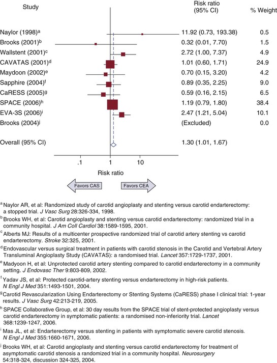
Figure 1-1 Example of a forest plot from a meta-analysis of carotid artery stenting (CAS) versus carotid endarterectomy (CEA) to determine 30-day risk for stroke and death. CI, Confidence interval. (Redrawn from Brahmanandam S, et al: Clinical results of carotid artery stenting compared with endarterectomy. J Vasc Surg 47:343-349, 2008.)
The strength of a meta-analysis comes from the strength of the studies that make up the composite variable. Furthermore, if available, the results of unpublished studies can also potentially influence the composite variable, because presumably many studies with nonsignificant results are not published. Therefore, an assessment of publication bias should be included with every meta-analysis. Publication bias can be assessed graphically by creating a funnel plot in which the effect size is compared with the sample size or other measure of variance. If no bias is present, the effect sizes should be balanced around the population mean effect size and decrease in variance with increasing sample size. If publication bias exists, part of the funnel plot will be sparse or empty of studies. Begg’s test for publication bias is a statistical test that represents the funnel plot’s graphic test.10 The variance of the effect estimate is divided by its standard error to give adjusted effect estimates with similar variance. Correlation is then tested between the adjusted effect size and the meta-analysis weight. An alternative method is Egger’s test, in which the study’s effect size divided by its standard error is regressed on 1/standard error.11 The intercept of this regression should equal zero, and testing for the statistical significance of nonzero intercepts should indicate publication bias.
Bias in Study Design
Clinical analysis is an attempt to estimate the “true” effects of a disease or its potential treatments. Because the true effects cannot be known with certainty, analytic results carry potential for error. All studies can be affected by two broadly defined types of error: random error and systematic error. Random error in clinical analysis comes from natural variation and can be handled with the statistical techniques covered later in this chapter. Systematic error, also known as bias, affects the results in one unintended direction and can threaten the validity of the study. Bias can be further categorized into three main groupings: selection bias, information bias, and confounding.
Selection bias occurs when the effect being tested differs among patients who participate in the study as opposed to those who do not. Because actual study participation involves a researcher’s determination of which patients are eligible for a study and then the patient’s agreement to participate in the study, the decision points can be affected by bias. One common form of selection bias is self-selection, in which patients who are healthier or sicker are more likely to participate in the study because of perceived self-benefit. Selection bias can also occur at the level of the researchers when they perceive potential study patients as being too sick and preferentially recruit healthy patients.
Information bias exists when the information collected in the study is erroneous. One example is the categorization of variables into discrete bins, as in the case of cigarette smoking. If smoking is categorized as only a yes or no variable, former smokers and current smokers with varying amounts of consumption will not be accurately categorized. Recall bias is another form of information bias that can occur particularly in case-control studies. For example, patients with abdominal aortic aneurysms may seemingly recall possible environmental factors that put them at risk for the disease. However, patients without aneurysms may not have a comparable imperative to stimulate memory of the same exposure.
Confounding is a significant factor in epidemiology and clinical analysis. Confounding exists when a second spurious variable (e.g., race/ethnicity) correlates with a primary independent variable (e.g., type 2 diabetes) and its associated dependent variable (e.g., critical limb ischemia). Researchers can conclude that patients in certain race/ethnicity groups are at greater risk for critical limb ischemia when diabetes is actually the stronger predictor. Confounding by indication is especially relevant in observational studies. This can occur when, without randomization, patients being treated with a drug can show worse clinical results than untreated counterparts because treated patients were presumably sicker at baseline and required the drug a priori. Confounding can be addressed by several methods: assigning confounders equally to the treatment and control groups (for case-control studies); matching confounders equally (for cohort studies); stratifying the results according to confounding groups; and multivariate analysis.
Outcomes Analysis
As physicians, we can usually see the natural progression of disease or the clinical outcome of treatment. Although these observations can be made for individual patients, general inferences about causation and broad application to all patients cannot be made without further analysis. Clinical analysis attempts to answer these questions by either observing or testing patients and their treatments. Because clinical analysis can be performed only on a subset or sample of the relevant entire population, a level of uncertainty will always exist in clinical analysis. Statistical methods are an integral aspect of clinical analysis because they help the researcher understand and accommodate the inherent uncertainty in a sample in comparison to the ideal population. In the following sections, common clinical analytic methods are reviewed so that the reader can better interpret clinical analysis and also have foundations to initiate an analysis. Reference to biostatistical and econometric texts is recommended for detailed derivation of the methods discussed.
Statistical Methods
At the beginning of most clinical analyses, descriptive statistics are used to quantify the study sample and its relevant clinical variables. Continuous variables (such as weight or age) are expressed as means or medians; categorical variables (such as the Trans-Atlantic Society Consensus [TASC] Classification: A, B, C, or D) are expressed as numbers or percentages of the total. Study sample characteristics and their relative distribution of comorbid conditions help determine whether the sample is consistent with known population characteristics, and hence, addresses the issue of generalizability of the clinical results to the overall population.
The next step in clinical analysis is hypothesis testing, in which the factor or treatment of interest is tested against a control group. The statistical methods used in hypothesis testing depend on the research question and characteristics of the data under comparison (Box 1-1). At its core, hypothesis testing asks whether the observable differences between groups represent a true difference or an apparent difference attributable to random error. A variety of statistical tests are available to accommodate the types of data being analyzed.
One major distinguishing characteristic of data is whether it fits a normal (or Gaussian) distribution, where the distribution of continuous values is symmetric and has a mean of 0 and a variance of 1. Gaussian distributions are one example of parametric data in which the form of the distribution is known. In contrast, nonparametric data are not symmetric around a mean, and the distribution of the data is not well known. Nonparametric statistical methods are thus used because fewer assumptions about the shape of the distribution are made. In general, nonparametric methods can be used for parametric data to increase robustness, but at a cost of statistical power. However, the use of parametric methods for nonparametric data or data containing small samples can lead to misleading results.
Regression Analysis
Among the statistical tests available, a few deserve special mention because of their common application to the clinical analysis of studies of vascular patients. Regression analysis is a mathematical technique in which the relationship between a dependent (or response) variable is modeled as a function of one or more independent variables, an intercept, and an error term. General linear models take the form Y = β0 + β1x1 + β2x2 + … + βnxn + e, although the model can take quadratic and higher functions of x and still be considered in the linear family. The coefficients (β1, β2, etc.) are model parameters calculated to “fit” the data, as commonly done with the least-squares method. They describe the magnitude of effect that each independent variable (x) has on the dependent variable (Y). The goodness of fit for the model is tested by using the R2 value and analysis of residuals. R2 is the proportion of variability that is accounted for by the model and has a range of 0 to 1. Although higher R2 values imply better fit, there is no defined threshold for goodness of fit, because R2 can be unintentionally increased by adding more variables to the model. For binary dependent variables, a logistic (logit) regression is used, whereas for continuous dependent variables, linear regression is used (Box 1-1).
Survival Analysis
Survival analysis is a statistical method used to evaluate death or failure as related to time. Key variables needed for analysis include event status (e.g., graft patency or failure, patient living or dead) and the timing of that status measurement. Survival analysis also incorporates censorship, in which data about the event of interest are unknown because of withdrawal of the patient from the study. Traditionally, in clinical analysis, “death” is the event variable, and “loss to follow-up” is the censorship variable. In vascular surgery, where graft patency is more often the endpoint of interest, “graft patency” is treated as the event variable and “death or study withdrawal” is treated as the combined censoring variable. This assumes that censorship (death) is not due to the event (loss of graft patency); however, this assumption cannot be held true in other fields, such as oncology (death attributable to failure of cancer treatment) or cardiac surgery (death caused by loss of coronary artery bypass graft patency).
In essence, survival analysis accounts for event status between fixed periods of measurement. For example, in traditional methods, if graft patency is measured only after 1 year, a graft that fails at 30 days is statistically treated the same as a graft that fails on day 364. Similarly, a graft that was patent at 360 days but was lost to follow-up is treated the same as a graft that was patent but lost to follow-up at 60 days. In contrast, life-tables measure events at fixed intervals (e.g., every 30 days), so occurrences before 365 days are accounted for (Fig. 1-2).12 Such analysis allows greater precision of events, but resolution is still limited to fixed time points. In the Kaplan-Meier (KM) method, each event is recorded at the time of occurrence, without the need for fixed time frames (Fig. 1-3).13 Although the KM method allows more precise analysis of events and censorship, life-tables are still appropriate when only predetermined periodic measurement of events is available or when arbitrary important milestones are of interest, such as 1-year graft patency or patient survival.
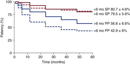
Figure 1-2 Example of life-table analysis of primary patency (PP) and secondary patency (SP) of bypass grafts after being revised before or after 6 months from the index operation. (Redrawn from Nguyen LL, et al: Infrainguinal vein bypass graft revision: factors affecting long-term outcome. J Vasc Surg 40:916-923, 2004.)
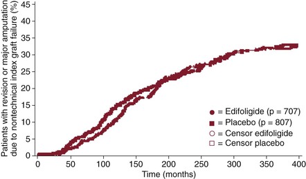
Figure 1-3 Example of Kaplan-Meier analysis of the effect of edifoligide on nontechnical graft failure. Each mark represents an event (graft failure) or censor (death or dropout). (Redrawn from Conte MS, et al: Results of PREVENT III: a multicenter, randomized trial of edifoligide for the prevention of vein graft failure in lower extremity bypass surgery. J Vasc Surg 43:742-751, discussion 751, 2006.)
The strength of survival analysis really lies in the ability to statistically account for censored data. The KM estimator (also known as the product-limit estimator) is the nonparametric maximum likelihood estimator of the survival function, which is based on the probability of an event conditional on reaching the time point of the previous event. The life-table method (or actuarial method) treats censored events as though they occurred at the midpoint of the time period. Most commonly, the Greenwood formula is used to calculate the standard error of the KM and life-table estimator for independent events.
Several tests are commonly used to test for differences between survival functions. The log-rank test adds observed and expected events within each group and sums them across all time points containing events. The log-rank statistic serves as the basis for the proportional hazard model (discussed later). In contrast, the Wilcoxon test is the log-rank test weighted by the number of patients at risk for each time point. Mathematically, the Wilcoxon test gives more weight to early time points and is thus less sensitive than the log-rank test to differences between groups that occur at later time points. Unlike the parametric log-rank and Wilcoxon tests, Cox proportional hazard models assume that the underlying hazard (risk) function is proportional over time, so that parameters can be estimated without compete knowledge of the hazard function. Other hazard models, such as the exponential, Weibull, or Gompertz distributions, instead assume knowledge of the hazard function. The Cox proportional hazard assumption allows the application of survival analysis techniques to multivariable models because individual hazards do not have to be specified for each independent variable in the model.
Propensity Scoring
Propensity scoring is a statistical method that seeks to control for confounding. It is used most often to control for confounding by indication, where patients have already been assigned a treatment based on unspecified reasons. For each patient, a propensity score is generated to reflect the conditional probability of being in a treatment group based on known variables. In essence, this balances the treatment groups to allow testing of the treatment effect and is analogous to randomization. Two common methods of obtaining balanced groups are available: trimming and reweighting. In trimming, patients at the extremes of the propensity score are eliminated from the analysis so that the remaining cohorts are more comparable matches. In reweighting, all patients are kept in the analysis, but their characteristics are reweighed to provide equivalency between groups.
Limitations of propensity methods include an inability to control for unknown confounders (a feat that RCTs manage). Furthermore, the variables used to create the propensity score must be carefully chosen to reflect potential predictors of treatment assignment, but not outcomes of assignment. Despite these drawbacks, when an RCT is not possible or practical, propensity scoring methods are useful for providing some insight in comparing treatment groups. Propensity score methods have also been used for other purposes, including nesting covariates for multivariable regression models and generation of reweighted estimating equations to rebalance weights from missing data.
Errors in Hypothesis Testing
The null hypothesis is the default position of no difference between two or more groups. Because the null hypothesis can never be proven, hypothesis testing can only reject or fail to reject the null hypothesis. Two types of errors can be made in hypothesis testing. A type I error is rejection of the null hypothesis when the null hypothesis is true. Alpha (α) is the probability of making a type I error. The P value is calculated from statistical testing and represents the probability of obtaining a result as extreme or more extreme than the results observed. Commonly, α is set at .05, and a P value less than α would reject the null hypothesis. Because α = .05 is an arbitrary setting, many will report actual P values to more precisely communicate statistical significance. Stricter α can be used when concern for a type I error is heightened, as in the testing of a large number of independent variables. For example, if 20 variables are tested, 1 variable (on average) is expected to be falsely positive with an α of .05. Accordingly, a stricter α of .01 or less may be required to reduce type I error. Conversely, a more relaxed α (typically .20) can be used in building stepwise regression models to be more inclusive of borderline variables.
A type II error is failure to reject the null hypothesis when the null hypothesis is false. Beta (β) is the probability of making a type II error. Power is defined as the probability of rejecting the null hypothesis when it is false (or concluding that the alternative hypothesis is true when it is true). In other words, power is the ability of a study to detect a true difference. Power is calculated as 1 − β and is closely related to sample size. Power analysis can be performed before or after data collection. A priori power analysis is used to determine the sample size needed to achieve adequate power for a study. Post hoc power analysis is used to determine the actual power of the study. Power analysis requires specification of several parameters, including α (usually .05), the level of power desired (usually 80%), expected effect size, and variance. Variance is simply estimated from previous measurements of related outcomes. However, the expected effect size is a parameter most susceptible to unintended influence. Setting the expected effect size too small decreases type I error, but also decreases power and results in the necessity of enrolling larger numbers of patients. Setting the expected effect size too large allows lower enrollment numbers, but at the cost of type I error. The actual calculation for necessary sample size depends on the expected statistical test for the data and can be performed by using “power calculators” available at statistics websites or with statistical software packages.
Statistical and Database Software
Before the widespread use of computers, statistics were calculated by hand through tedious procedures. Statistical software and computing power have greatly improved the ability and efficiency of statisticians and clinical researchers. Even the rapid advancements in desktop computing ability in the last decade have resulted in faster analysis of larger amounts of data via more complex modeling. At its core, statistical software requires user coding of specific commands to perform data analysis and database manipulation. SAS (originally Statistical Analysis System) was created by Anthony Barr from his work as a graduate student at North Carolina State University in the early 1960s. He and other collaborators later created the SAS Institute in 1976 to commercialize the statistical package. SAS statistical software is widely used in clinical analysis of large trials, epidemiology, the insurance industry, and other business applications of data mining. Frequently, the development of new statistical techniques is included as new SAS commands or macros. Stata was created by Statacorp and is the other widely used statistical program, especially in the social sciences and economics. Stata can open only one data set at a time and hold it in virtual memory, which can limit its use for very large data sets.
Both SAS and Stata also have graphics user interfaces (GUIs) that automate or facilitate statistical analysis without exposing the user to the complexities of coding, although most users of these packages prefer the native coding interface. Most other statistical packages, such as SPSS (originally Statistical Package for the Social Sciences), JMP, and Minitab, are promoted with GUIs and pulldown menus as the primary interface for performing statistical tests. Another statistical package that is rapidly gaining in popularity is R, particularly because it is both free and highly functional. It is available with only a very limited GUI. However, others have created more elaborate GUIs that are available for download. We do not recommend one product over another, but do recommend that clinical researchers be familiar with at least one of these widely used packages. The choice often depends on the preferences of the local institution or research field. For those so inclined, direct statistical coding allows greater flexibility and creativity in data analysis and modeling than GUIs can provide. Even when clinicians rely on full-time statisticians to perform the analysis, detailed interpretation of raw statistical output requires some basic knowledge of the statistical software used to generate the results.
Functional Studies
Traditionally, the ankle-brachial index (ABI) has been widely used to screen for peripheral vascular disease and to quantify its severity. ABI has also been correlated with walking ability, quality of life (QoL),14 and cardiovascular comorbidity.15 In addition, ABI has been used as a measure of success in PAD revascularization. Despite its utility, ABI does not directly measure PAD functional performance, namely, walking performance in claudication patients. Furthermore, traditional ABI measurements are obtained from patients at rest in the supine position rather than during activity, where tissue demand, increased cardiac output, and vasodilatation may alter ABI measurements. Treadmills were first used to diagnose and evaluate cardiopulmonary function, but have since been applied to walking performance as well. Patients are asked to walk on the treadmill, and their claudication pain distance and maximal walking distance are recorded. Constant-load exercise testing consists of a fixed speed and treadmill grade, whereas in graded treadmill testing, the slope is increased at each interval (e.g., 2% grade every 2 minutes). Graded testing has the advantage of a broader range of walking challenge to patients and increases the likelihood that they will reach their claudication pain distance and maximal walking distance within testing times. Because being in a walking program itself is associated with improved walking performance, frequent treadmill testing must have appropriate controls to better distinguish the treatment effect being studied.
Many elderly or disabled patients are uncomfortable or unable to walk on a treadmill where parameters such as speed and incline are predetermined. The 6-minute walking test was initially designed to test the functional capacity of patients with chronic congestive heart failure,16 but it has now been extended to test patients with claudication17 and other cardiopulmonary processes. Patients are asked to walk for 6 minutes at their own pace on level ground and with periodic resting if needed. This allows patients to control their walking speed and allows them to better demonstrate their real-life walking ability. Recently, global positioning satellite (GPS) monitors have been used to assess walking distance and speed during a dedicated outdoor walk.18 This new technology allows remote testing of patients and may be a more realistic reflection of their walking capability.
Quality of Life
Quality of life is the degree of wellness felt by an individual. QoL is generally considered a composite of two broadly defined domains: physical and psychological. Although the components of each domain can be measured, each individual patient’s overall QoL cannot be predicted because the effects are not necessarily similar among individuals. However, one can assume that for populations, higher physical and psychological domains generally lead to higher QoL. Health-related QoL (HRQoL) measures focus on health-related physical and psychological attributes, although it can be hard to isolate non–health-related factors influencing overall QoL.
Because QoL cannot be measured directly, surveys (also known as instruments) are used to obtain necessary information. When compared with other clinical methods, surveys have low cost and allow efficient collection of information from a large number of participants. However, surveys are susceptible to variability in response as a result of temporary motivational states, cultural and language differences, and other impairments affecting survey completion. Several instruments have been developed for both specific disease fields and for general applicability. Instruments cannot be developed to suit specific needs without undergoing validity and reliability testing. Validity is the degree to which an instrument measures what it was intended to measure. Validity has several aspects, including the ability of the instrument to support the causal effect being tested (internal validity), generalize the effect to the larger population from which the sample was drawn (statistical validity), support the intended interpretation of the effect (construct validity), and support the generalization of results to external populations (external validity). Reliability is the consistency of the instrument if it were to be repeated on the same participant under identical conditions. Reliability can be tested by multiple administration of the test to the same participant or by single administration of the test to a divided participant population. Reliability does not imply validity because an instrument can measure an effect consistently, but that effect may not be the causal effect being studied. Reliability is analogous to precision, whereas validity is analogous to accuracy.
Health-Related, Quality-of-Life Survey Instruments
Types of Survey Instruments.
The Short Form (36 questions) Health Survey (SF-36) is perhaps the best known HRQoL instrument; it has been used in more than 4000 medical publications, applied to 200 different diseases and conditions, and translated for use in 22 different countries. The SF-36 consists of 36 questions that yield an eight-scale profile of functional healing and well-being.19 The physical component summary is composed of physical functioning, role (physical), body pain, and general health, whereas the mental component summary is composed of vitality, social functioning, role (emotional), and mental health. In 1996, SF-36v2 was released with modifications in wording, layout, response scales, scoring, and expected norms. The SF-12 (and now the SF-12v2) is a subset of SF-36 that still measures the eight health domains. Its brevity is ideal for use in conjunction with longer disease-specific instruments. The SF-8 was designed to measure the eight health domains through single questions for each domain. It was created by using information from various questionnaires, including, but not limited to, SF-36. However, the SF-8 was calibrated with the same metric as the SF-36, and thus, the summary scores can be compared. The SF-36 was developed without utility measures (detailed in the next section), but algorithms have been developed to address this shortcoming.
The EQ-5D was developed by the European Quality of Life Group (EuroQol) as a non–disease-specific instrument for describing and valuing HRQoL.20 It is designed to be cognitively simple, quick to complete, and easily self-administered. Currently, the EQ-5D is available in 160 languages. The EQ-5D consists of a descriptive system composed of five dimensions of health: mobility, self-care, usual activities, pain and/or discomfort, and anxiety and/or depression. A health state is generated from these dimensions and then converted into a weighted health state index by applying scores from the EQ-5D value sets generated from general population samples. The EQ-5D also has a visual analog scale component that records the patient’s self-rated health status on a vertical graduated (0 to 100) scale. The visual analog scale serves as the utility measure that allows conversion of the results for use in decision and cost-effectiveness analysis.
The Walking Impairment Questionnaire (WIQ) is a four-component instrument designed to assess walking performance in claudicants.21 A score is generated for each of the four components: walking distance, walking speed, stair climbing, and other symptoms that may limit walking. The WIQ has been correlated with treadmill walking time and validated in patients with and without PAD. It uses “blocks” as a measure of distance and “flight of stairs” as a measurement of stair climbing, measures that may not be applicable to some cultures. Furthermore, the lack of utility measures in WIQ limits its use in advanced QoL analysis. Nevertheless, as a survey instrument, the WIQ functions well as a gauge of walking performance in patients undergoing treatment for claudication.
The Vascular Quality of Life Questionnaire (VascuQol) was developed at King’s College Hospital, London, to assess patients with chronic lower extremity ischemia rather than just claudication.22 The questionnaire contains 25 questions divided into 5 domains: pain, symptoms, activity, social, and emotional. Validity and test-retest reliability were evaluated and found to be very high. Continued use of this relatively new instrument will provide additional confirmation of its role in QoL analysis.
Limitations of Survey Instruments.
All surveys have unique concerns that need to be addressed by researchers. One of the biggest is incomplete surveys. Because surveys are usually administered before and after a treatment or observation period, the absence of a survey for some patients during follow-up periods is troublesome. Although many researchers simply include only patients with complete surveys, this strategy may introduce bias into the results. The most severe case of omission bias is due to the fact that dead study patients cannot complete surveys. For more subtle factors, complex regression analysis of patients with missing data can identify potential factors associated with survey incompletion and serve as a cautionary measure against over-interpretation of results. A second issue in surveys is the statistical challenge of repeated measures. Because patients serve as their own survey control, simple pooled statistical techniques can mask individual effects. Mean differences, ratios, or preferably, paired tests must be used. When surveys are administered at three or more time points, simple one-to-one point comparisons do not completely account for the relationships between all time points. Linear mixed-method regression modeling can be adapted for multiple repeated measures to control for missing data.23
Economic Analysis
The conduct of health care occurs in the context of perceived patient benefits and incurred societal costs. For example, bypass graft or stent patency is not the only endpoint in the care of claudication. Rather, it is an important contributor of the patient’s ambulatory status, which, in turn, influences overall QoL. This care has a cost to society, but it can also result in benefit to society in the form of intellectual and labor contributions made by the treated patient. Therefore, analysis of clinical outcomes should be made in the framework of its impact on the patient, the health care system, and society.
Utility Measures
In economic analysis and decision analysis, patients are considered to be in distinct “states” that reflect defined medical diagnoses or symptoms (e.g., asymptomatic vs symptomatic carotid artery stenosis). QoL instruments capture health states, but generally do not capture preferences for a given state. Utility measures capture how a person values (or prefers) a state of health, not just the characteristics of that state. Utility measures also have mathematical properties that allow their use in decision trees and cost-effectiveness analysis. The Health Utilities Index and the EQ-5D are two widely used utility measures. The simplest method of determining utility is to ask patients to value their own health or a hypothetical state of health by using a rating scale. This information is then transformed into a utility measure by using data from a reference population. Transformations of health states from descriptive instruments (e.g., SF-36) have also been created, although low correlations between descriptive and preference measures have been demonstrated. For transformations to be meaningful, the reference population itself has to be subject to utility assessment.
Direct assessment of utility can be performed by using the standard gamble, in which for a given health state, patients are asked whether they would choose to remain in that state or take a gamble between death and perfect health. The question is then repeated with varying gamble probabilities. The utility of the health state is then derived from the probability of achieving perfect health when the patient is at equilibrium (or indifferent between the choices) between taking the gamble or remaining in the known state of intermediate health. Another common direct utility assessment method is the time tradeoff, in which the patient is asked to choose between a length of life in a given compromised state and a shorter length of life in a perfect state. The utility of the health state is then derived from the ratio of the shorter to the longer life expectancy at the point of equilibrium.
Because these utility assessment methods are artificial and do not actually expose subjects to decisions with true implications, variations in utility values exist between the methods. Generally, standard gamble methods generate the highest utility values because most patients are unwilling to accept a significant risk of sudden death, even if the alternative health state is poor. Utility values from time tradeoff methods are lower, which is consistent with the theory that decreased life expectancy is an easier price to pay for a chance to improve health. Rating scales usually generate the lowest utility values because there is no perceived penalty for underrating, as there is with the other methods.
Decision Analysis
In the daily practice of surgery, many significant decisions involve tradeoffs between risk and benefit with uncertainties. Uncertainties can exist with diagnostic testing, the actual diagnosis, the natural history of the disease, and the treatment choices and their outcomes. Despite these uncertainties, a decision must be made. Decision analysis is the formal methodology of addressing decisions by defining the problem, considering alternative choices, modeling the consequences, and estimating their chances. The process not only reveals the best choices for a particular type of patient, but also demonstrates the critical factors that may alter that decision. Thus, for the practicing clinician, knowledge of relevant decision analyses may serve as a foundation from which to make decisions and as a resource with which to modify that decision based on patient specifics.
One of the primary tools used in decision analysis is the decision tree, where the relevant factors are represented in chronological relationship to each other from left to right. The alternative choices (diagnostic tests, natural history states, treatments, etc.) are visually represented on branches of the tree, and each branch point is a decision node (usually represented as a square) in which a choice is possible, or a chance node (usually represented as a circle) in which the probability of a consequence is conditional on the events that preceded it. The end of each branch has an outcome that is based on the choices made preceding it and their probabilities. Each outcome is then given a value, whether it is life expectancy, quality-adjusted life-years (QALYs), or cost. The expected value for each alternative is then calculated on the basis of cumulative probabilities and outcome values. The best decision is then chosen to optimize the outcome value, such as the lowest cost or highest QALYs.
The results from decision analysis are strongly influenced by the event probabilities and outcome values used. Ideally, these figures are derived from strong clinical studies in the field, although a consensus on precise figures and values can be difficult. Sensitivity and threshold analysis can then be performed to test the results of decision analysis under different probability and outcome assumptions. Sensitivity analysis is performed mathematically by setting the key probability as an unknown variable to be solved algebraically. This results in a probability value threshold around which the analysis can change to favor different decisions. If the threshold value (or probability) is within accepted estimated clinical probabilities for that event, researchers can have greater confidence in the applicability of the decision analysis results.
Markov Models and Monte Carlo Simulation
The decision trees discussed in the previous section work well for clinical situations in which one or a small number of decisions are made over a defined time frame. In reality, decision points may occur repeatedly, and the relevant factors influencing the outcome may also change over time. Markov models (named after the Russian mathematician Andrey Markov) assume that patients begin in one of a discrete number of possible mutually exclusive “states.” For every cycle, each patient has a probability of remaining in the state or transitioning between one state and the next. Markov models also assume the Markov property, whereby future states are independent of past states. The model can then be analyzed by using matrixes, cohort simulation, or Monte Carlo simulation. Matrix solutions require matrix algebra techniques and can be used only when transition probabilities do not vary over time, and costs are not discounted. Cohort simulation begins with a hypothetical large cohort of patients and subjects them to the Markov transition probabilities. A table is then generated with the new cohort distribution among the states. The process is repeated for the next and subsequent cycles until there is equilibrium or all patients are in a state without an exit, called the absorbing state. Monte Carlo simulation is similar to cohort simulation, except that one patient at a time is simulated, rather than the entire cohort. The simulation continues until the patient arrives at the absorbing state, or the predetermined cycle is reached in models without absorbing states. Simulation of individual patients allows researchers to measure the variance of outcomes in addition to the mean.
Cost Benefit and Cost-Effectiveness Analysis
At the heart of cost analysis is the assumption that resources are constrained. If unlimited resources are available, all testing and treatment would be offered, as long as they are not harmful. However, in an environment of limited resources, cost analysis helps policymakers and clinicians decide on the greatest utility of the resources available. Cost analysis is certainly not the only or necessarily the best criterion for making health policy decisions, but it is an objective, quantitative tool that yields important information about the efficacy of clinical practice, and thus, may serve as a key factor in the overall choice of health care decisions.
From an economic standpoint, tests or treatments can be measured in two parameters: health improvement and cost saving. Treatments that improve health and save cost are considered superior and should be adopted. Likewise, treatments that do not change (or worsen) health and increase cost should be abandoned. Treatments that improve health but also increase cost or do not change health but decrease cost need further investigation before implementation. Cost-effectiveness analysis (CEA) compares treatments based on a common measure of cost and health effectiveness. The measure of health effectiveness can be represented by the number of lives saved, cases cured, cases prevented, and preference-based utility measures such as QALYs. Cost-benefit analysis (CBA) seeks to quantify cost and health effectiveness in monetary terms, with positive CBA treatments being favored over those with negative CBA. CBA is useful for comparing very different choices of treatments or interventions. Because many involved in health care are uncomfortable with the monetary valuation of life and life-years, CEA is more commonly used in health-related analysis, whereas CBA is more prevalent in economic-oriented health care analysis.
The CEA measure is the ratio of cost to effectiveness, typically dollars per QALY gained. Comparative choices (treatments, programs, tests) are subsequently ranked in order of lowest cost-effectiveness ratio to highest. Funding is then given to the programs with lowest cost per efficacy measure until all available funding is spent. The cost-effectiveness ratio of the last funded program in this algorithm is defined as the permissible cost-effectiveness threshold for other programs to meet until new budgetary constraints are in effect. In the United Kingdom, the National Institute for Health and Clinical Excellence has adopted a cost-effectiveness threshold range of £20,000 to £30,000 ($39,400 to $59,100 U.S. dollars) per QALY gained. In the United States, no official threshold has been adopted, although many in practice have used the threshold of $60,000 per QALY. This figure is based on the calculated average cost of hemodialysis per person per year and Medicare’s special coverage of renal failure patients, regardless of age.
The term cost is often misunderstood and misused. In economic analysis, cost is not limited to currency but can be applied to other valuable resources, such as time, personnel, space, and alternative choices. Opportunity cost is the loss or sacrifice incurred when one mutually exclusive option is chosen over another. Thus, if a plot of land is chosen to be developed into a hospital, the cost of that project includes the building cost, as well as the lost opportunity to build a different facility at that site. Cost must also be distinguished from “charges” by health care researchers because administrative accounting data often contain billing charges, which are based on the cost of materials and services, but probably also include indirect costs and a margin for profit. For most health care cost analyses, cost is stated from the perspective of the society. This utilitarian perspective differs from the perspective of the patient, provider, and institution. Although these other perspectives have validity, the societal perspective is more comprehensive and eliminates distortions, such as moral hazard and cost shifting.
Outcomes Translational Research
The practice of surgery has undergone several important transformations since its early beginnings. Initially, issues of anatomy, physiology, and anesthesia were the obstacles to overcome for advancement of the field. Adoption of technology and refinement of surgical technique helped define the growth of surgery in the last century. Most recently, study of clinical outcomes plus adherence to evidence-based medicine has increased the efficacy and safety of surgery. The proliferation of surgical care (and medicine as a whole) does come with a cost, however. In the United States, expenditure on health care for 2011 was $2.7 trillion, which corresponds to $8680 per person or 17.9% of the gross national product. Other developed countries spend less, but their expenditures are increasing.
Although the actual care of patients will continue to challenge us, the way we conduct and finance health care will also have a profound impact. Thus, health care is a continuum from advancements in basic sciences, to patient applications, to clinical outcomes, to efficacy analysis, and finally, to policy. Translational research has been coined to describe the connection between the basic sciences and patient care. Similarly, outcomes translational research can be thought of as the connection between clinical outcomes and health care policy. Policy decisions based on arbitrary expenditure caps may be an effective way to control health care costs, but the resulting distribution of resources may be inefficient. Rather, policy should be based on clinical evidence and efficacy so that limited resources are used optimally.
Outcomes translational research begins with careful analysis of clinical results. Such analysis should ideally incorporate carefully designed studies to understand the natural history of disease and compare treatment options. Even the outcome measure itself needs thoughtful selection. For example, in the surgical treatment of claudication, the classic measure of outcome was bypass graft patency. With the greater adoption of percutaneous treatment methods, vessel patency has been adopted. However, vessel patency does not accurately reflect all outcomes. From the patient’s perspective, improvement in walking function (and its effect on QoL) is the benchmark. Although vessel patency clearly influences walking function, a patent vessel does not confer improved walking if other comorbid conditions, such as severe arthritis or neuropathy, are limiting. Conversely, assessment of functional and QoL endpoints alone does not allow analysis of the components leading to patient-perceived improvements. Greater understanding of technical success, vessel patency, and treatment durability will allow further improvements in the treatments themselves. Therefore, measurement of clinical outcomes is a multimodality technique involving the use of integrated components that measure several aspects of success and failure.
There is no doubt that the results of clinical trials have had an impact on the care of surgical patients. However, these trials are costly and may not have comprehensive generalizability because most trials occur in large institutions with known expertise in the area of interest. The majority of vascular surgery occurs outside clinical trials, in institutions of varying size, and by practitioners of varying expertise. The outcomes of these “real-world” efforts are not well studied. Many have used large national or statewide administrative databases in an attempt to analyze care broadly, although these databases lack detailed information because they were not designed to be research tools. For example, most administrative databases do not distinguish the left from the right extremity. Thus, two vascular procedures performed on an extremity within 1 year can be a revision of the first procedure, or they can signify sequential bilateral procedures. Other surgical and medical specialties have comprehensive registries that allow broader inclusion of patients who receive care within specific diagnostic groups. In the field of vascular surgery, other countries have national registries with research and administrative objectives. In the United States, efforts are under way to extend statewide or regional databases to encompass a wider cohort. The cost of such endeavors is certainly a factor in achieving a nationwide database, although arguably, the cost of not knowing the outcomes and efficacy of health care may be greater.
The use of economic analysis is an important component of outcomes translational research because health care, like all human effort, requires resources. Economics has often been maligned as being “cold,” and this quality is its strength, not its weakness. Few of us can hope to be without bias when making health care decisions for ourselves, our patients, or our relatives. By extension, each specialty group strives to increase resources that can be applied to their disease or cause. Economic analysis of health care allows assessment of outcomes as measured by a common comparable unit (cost). However, economics as a whole can shed light only on the tradeoffs between different alternatives and their impact. It is up to policymakers to assign value to these tradeoffs, and in the end, make decisions about allocation of health care resources. In some ethical and societal frameworks, additional value may be assigned to the treatment of specific disease groups (e.g., dialysis care) that is not captured by traditional analytic methods. Nevertheless, without clinical and economic analytic tools, such decisions are made while blinded to their impact on alternative decisions. Clinician researchers in outcomes translational research are well suited to contribute to the policies that affect health care because they can generate data to help formulate policy and also see the effect of policy on the individual patients they are treating.
Selected Key References
Freedman B. Equipoise and the ethics of clinical research. N Engl J Med. 1987;317:141–145.
Ethics of clinical research.
Rabin R, de Charro F. EQ-5D: A measure of health status from the EuroQol Group. Ann Med. 2001;33:337–343.
EQ-5D reference.
Regensteiner JG, Steiner JF, Panzer RJ, Hiatt WR. Evaluation of walking impairment by questionnaire in patients with peripheral arterial disease. J Vasc Med Biol. 1990;2:142–150.
Functional evaluation of PAD.
Stroup DF, Berlin JA, Morton SC, Olkin I, Williamson GD, Rennie D, Moher D, Becker BJ, Sipe TA, Thacker SB. Meta-analysis of observational studies in epidemiology: a proposal for reporting. Meta-analysis Of Observational Studies in Epidemiology (MOOSE) group. JAMA. 2000;283:2008–2012.
Standards for meta-analysis of observational studies.
Ware JE Jr, Sherbourne CD. The MOS 36-item short-form health survey (SF-36). I. Conceptual framework and item selection. Med Care. 1992;30:473–483.
SF-36 reference.
The reference list can be found on the companion Expert Consult website at www.expertconsult.com.
References
1. Eyler JM. The changing assessments of John Snow’s and William Farr’s cholera studies. Soz Praventivmed. 2001;46:225–232.
2. Haynes RB, et al. Transferring evidence from research into practice: 1. The role of clinical care research evidence in clinical decisions. ACP J Club. 1996;125:A14–A16.
3. Dawber TR, et al. The Framingham Study. An epidemiological approach to coronary heart disease. Circulation. 1966;34:553–555.
4. Kannel WB, et al. Cigarette smoking and risk of coronary heart disease. Epidemiologic clues to pathogenesis. The Framingham Study. Natl Cancer Inst Monogr. 1968;28:9–20.
5. Freedman B. Equipoise and the ethics of clinical research. N Engl J Med. 1987;317:141–145.
6. Smith GC, et al. Parachute use to prevent death and major trauma related to gravitational challenge: systematic review of randomised controlled trials. BMJ. 2003;327:1459–1461.
7. Smith ML, et al. Meta-analysis of psychotherapy outcome studies. Am Psychol. 1977;32:752–760.
8. Stroup DF, et al. Meta-analysis of observational studies in epidemiology: a proposal for reporting. Meta-analysis Of Observational Studies in Epidemiology (MOOSE) group. JAMA. 2000;283:2008–2012.
9. Jones DR. Meta-analysis of observational epidemiological studies: a review. J R Soc Med. 1992;85:165–168.
10. Begg CB, et al. Operating characteristics of a rank correlation test for publication bias. Biometrics. 1994;50:1088–1101.
11. Egger M, et al. Bias in meta-analysis detected by a simple, graphical test. BMJ. 1997;315:629–634.
12. Nguyen LL, et al. Infrainguinal vein bypass graft revision: factors affecting long-term outcome. J Vasc Surg. 2004;40:916–923.
13. Conte MS, et al. Results of PREVENT III: a multicenter, randomized trial of edifoligide for the prevention of vein graft failure in lower extremity bypass surgery. J Vasc Surg. 2006;43:742–751.
14. McDermott MM, et al. Leg symptoms, the ankle-brachial index, and walking ability in patients with peripheral arterial disease. J Gen Intern Med. 1999;14:173–181.
15. Allison MA, et al. A high ankle-brachial index is associated with increased cardiovascular disease morbidity and lower quality of life. J Am Coll Cardiol. 2008;51:1292–1298.
16. Guyatt GH, et al. The 6-minute walk: a new measure of exercise capacity in patients with chronic heart failure. Can Med Assoc J. 1985;132:919–923.
17. Montgomery PS, et al. The clinical utility of a six-minute walk test in peripheral arterial occlusive disease patients. J Am Geriatr Soc. 1998;46:706–711.
18. Le Faucheur A, et al. Measurement of walking distance and speed in patients with peripheral arterial disease: a novel method using a global positioning system. Circulation. 2008;117:897–904.
19. Ware JE Jr, et al. The MOS 36-item short-form health survey (SF-36). I. Conceptual framework and item selection. Med Care. 1992;30:473–483.
20. Rabin R, et al. EQ-5D: a measure of health status from the EuroQol Group. Ann Med. 2001;33:337–343.
21. Regensteiner JG, et al. Evaluation of walking impairment by questionnaire in patients with peripheral arterial disease. J Vasc Med Biol. 1990;2:142–150.
22. Morgan MB, et al. Developing the Vascular Quality of Life Questionnaire: a new disease-specific quality of life measure for use in lower limb ischemia. J Vasc Surg. 2001;33:679–687.
23. Nguyen LL, et al. Prospective multicenter study of quality of life before and after lower extremity vein bypass in 1404 patients with critical limb ischemia. J Vasc Surg. 2006;44:977–983.
[/level-membership-for-surgery-category][not-level-membership-for-surgery-category]Chapter 1
Epidemiology and Clinical Analysis
Louis L. Nguyen, Ann DeBord Smith
The goal of this chapter is to introduce the vascular surgeon to the principles that underlie the design, conduct, and interpretation of clinical research. Disease-specific outcomes otherwise detailed in subsequent chapters will not be covered here. Rather, this chapter discusses the historical context, current methodology, and future developments in epidemiology, clinical research, and outcomes analysis. This chapter serves as a foundation for clinicians to better interpret clinical results and as a guide for researchers to further expand clinical analysis.
Epidemiology
Epidemiology is derived from the Greek terms for “upon” (epi), “the people” (demos), and “study” (logos), and can be translated into “the study of what is upon the people.” It exists to answer the four major questions of medicine: diagnosis, etiology, treatment, and prognosis.
Brief History
Hippocrates is considered to be among the earliest recorded epidemiologists because he treated disease as both a group event and an individual occurrence. His greatest contribution to epidemiology was the linkage of external factors (climate, diet, and living conditions) with explanations for disease. Before widespread adoption of the scientific method, early physicians inferred disease causality through careful observation. For example, they observed the geographic distribution of cases or common factors shared by diseased versus healthy persons. John Snow is recognized for ameliorating the cholera epidemic in the Soho district of London in 1854 by identifying the cause of the outbreak through mapping the location of known cases of cholera in the district. Based on the density and geographic distribution of cases, he concluded that the public water pump was the source and had the pump handle removed.1
Modern Developments
Modern epidemiology and clinical analysis seek to establish causation through study design and statistical analysis. Carefully designed studies and analyses can minimize the risk of false conclusions and maximize the opportunity to find causation when it is present. In other areas of biology, causation can be demonstrated by fulfilling criteria, such as Koch’s postulates for establishing the relationship between microbe and disease. In epidemiology, the study design that would offer ideal proof of causation would be comparison of people with themselves in both the exposed and the unexposed state. This impossible and unethical experiment would control for everything, except the exposure, and thus, establish the causality between exposure and disease. Because this condition cannot exist, it is referred to as counterfactual. Because the ideal study is impossible to conduct, alternative study designs have developed with different risks and benefits. The crossover experimental design, for example, approaches the counterfactual ideal by exposing patients to both treatment groups in sequence. However, the influence of time and previous exposure to the other treatment assignment may still affect the outcome (also known as the carryover effect). Other study designs exist that include techniques such as randomization or prospective data gathering to minimize bias. Appropriate study design must be selected based upon a study’s objectives. After a study is complete, conclusions can be drawn from a carefully crafted statistical analysis. Modern epidemiology includes applied mathematical methods to quantify observations and draw inferences about their relationships.
Evidence-based medicine is a relatively modern approach to the practice of medicine that aims to qualify and encourage the use of currently available clinical evidence to support a particular treatment paradigm. This practice encourages the integration of an individual practitioner’s clinical expertise with the best currently available recommendations from clinical research studies.2 Relying on personal experience alone could lead to biased decisions, whereas relying solely on results from clinical research studies could lead to inflexible policies. Evidence-based medicine stratifies the strength of the evidence from clinical research studies based on study design and statistical findings (Table 1-1). The criteria differ when the evidence is sufficient to support a specific therapeutic approach, prognosis, diagnosis, or other health services research. Criteria also differ among research institutions, including the U.S. Preventive Services Task Force and the U.K. National Health Service. However, common themes can be seen among the different fields. Systematic reviews with homogeneity are preferred over single reports, whereas randomized controlled trials (RCTs) are preferred over cohort and case-control studies. Even within similar study design groupings, the statistical strength of each study is evaluated, with preference for studies with large numbers, complete and thorough follow-up, and results with small confidence intervals. Clinical recommendations are then based on the available evidence and are further graded according to their strengths (Table 1-2).
Table 1-1
Levels of Evidence for Therapeutics
| Level | Evidence |
| 1a | Systematic reviews of RCT studies with homogeneity |
| 1b | Individual RCT with narrow confidence intervals |
| 1c | “All or none” trials* |
| 2a | Systematic reviews of cohort studies with homogeneity |
| 2b | Individual cohort studies |
| 2c | Clinical outcomes studies |
| 3a | Systemic reviews of case-control studies with homogeneity |
| 3b | Individual case-control studies |
| 4 | Case-series studies |
| 5 | Expert opinion without critical appraisal or based on bench research |
* In which all patients died before the therapeutic became available, but some now survive with it, or in which some patients survived before the therapeutic became available, but now none die with it.
RCT, Randomized controlled trial.
Adapted from Oxford Centre for Evidence-based Medicine (2001).
Table 1-2
Grades of Recommendation
| Grade | Recommendation | Basis |
| A | Strong evidence to support practice | Consistent level 1 studies |
| B | Fair evidence to support practice | Consistent level 2 or 3 studies or extrapolations from level 1 studies |
| C | Evidence too close to make a general recommendation | Level 4 studies or extrapolation from level 2 or 3 studies |
| D | Evidence insufficient or conflicting to make a general recommendation | Level 5 evidence or inconsistent studies of any level |
Adapted from U.S. Preventive Services Task Force Ratings (2003) and Oxford Centre for Evidence-based Medicine (2001).
Clinical Research Methods
Although measuring the incidence and prevalence of disease is useful in the initial understanding of a disease process, additional techniques must be used to identify risk factors and test treatments for disease. The choice of study design and statistical analysis technique depends on the available data, the hypothesis being tested, and patient safety and/or ethical concerns.
Study Design
Clinical research can be broadly divided into observational studies and experimental studies. Observational studies are characterized by the absence of a study-directed intervention, whereas experimental studies involve testing a treatment, be it a drug, a device, or a clinical pathway. Observational studies can follow ongoing treatments but cannot influence choices made in the treatment of a patient. Observational studies can be executed in a prospective or retrospective fashion, whereas experimental studies can be performed only prospectively.
Two factors that affect choice of study design include prevalence and incidence of disease. The prevalence of disease is the ratio of persons affected for the population at risk and reflects the frequency of the disease at the measured time point, regardless of the time of disease development. In contrast, the incidence is the ratio of persons in whom the disease develops within a specified period for the population at risk. For diseases with short duration or high mortality, prevalence may not accurately reflect the impact of disease because the single time point of measurement does not capture resolved disease or patients who died of the disease. Prevalence is a more useful parameter when discussing diseases of longer duration, whereas incidence is more useful for diseases of shorter duration.
Observational Studies
There are two main types of observational studies: cohort and case-control studies. A cohort is a designated group of individuals that is followed over a period of time. Cohort studies seek to identify a population at risk for the disease of interest. After a period of observation, patients in whom the disease develops are compared with the population of patients who are free of the disease. Cohort studies are most often associated with epidemiology because they comprise many of the most prominent studies in the modern era. The classic example is the Framingham Heart Study (FHS), in which 5209 residents of Framingham, Massachusetts, were monitored prospectively, starting in 1948.3 Much of our epidemiologic knowledge regarding risk factors for heart disease comes from the FHS.4 Although the FHS was initially intended to last 20 years, the study has subsequently been extended and now involves the third generation of participants. Cohort studies also seek to identify potential risk factors for development of the disease of interest. For example, if cigarette smoking is suspected in the development of peripheral arterial disease (PAD), smokers are assessed for the development of PAD from the beginning of the observation period to the end of the observation period. Because PAD does not develop in all smokers, and conversely, not all PAD patients are smokers, a relative risk (RR) is calculated as the ratio of the incidence of PAD in smokers versus the incidence of PAD in nonsmokers.
The main challenge in case-control studies is to identify an appropriate control group with characteristics similar to those of the general population at risk for the disease. Inappropriate selection of the control group may lead to the introduction of additional confounding and bias. For example, matched case-control studies aim to identify a control group “matched” for factors found in the exposure group. Unfortunately, by matching even basic demographic factors, such as gender and the prevalence of comorbid conditions, unknown co-associated factors can also be included in the control group and may affect the relationship of the primary factor to the outcome. Appropriate selection of the control group can be achieved by using broad criteria, such as time, treatment at the same institution, age boundaries, and gender when the exposure group consists of only one gender.
Experimental Studies
Experimental studies differ from observational studies in that the former expose patients to a treatment being tested. Many experimental trials involve randomization of patients to the treatment group or appropriate control group. Although randomization ensures that known factors are evenly distributed between the exposure and control groups, the importance of RCTs lies in the even distribution of unknown factors. Thus, a well-designed RCT will result in more simplified endpoint analyses because complex statistical models are not necessary to control for confounding factors.
Randomization can be accomplished by complete randomization of the entire study population, by block randomization, or by adaptive randomization. For complete randomization, each new patient is randomized without prior influence on previously enrolled patients. The expected outcome at the completion of the trial is an equal distribution of patients within each treatment group, although unequal distribution may occur by chance, especially in small trials. Block randomization creates repeated blocks of patients in which equal distribution between treatment groups is enforced within each block. Block randomization ensures better end randomization and periodic randomization during the trial. End randomization is important in studies with long enrollment times or in multi-institutional studies that may have different local populations. Because the assignment of early patients within each block influences the assignment of later patients, block randomization should occur in a blinded fashion to avoid bias. Intrablock correlation must also be tested in the final analysis of the data. Adaptive randomization seeks to achieve balance of assignment of randomization for a prespecified factor (e.g., gender or previous treatment) suspected of affecting the treatment outcome. In theory, randomization controls for these factors, but unique situations may require stricter balance.
RCTs can be classified according to knowledge of the randomization assignment by the treating clinicians and their patients. In open trials, the clinician and patients know the full details of the treatment assignment. This leaves the potential for bias in interpretation of results and may also influence study patients to drop out if they are randomized to a treatment group that they perceive to be unfavorable. Open trials are often conducted for surgical patients, where it is not possible or ethical to conceal the treatment assignment from the patient or the provider. In single-blinded trials, the clinician is aware of the treatment assignment, but the patient is not. These studies have more effective controls, but are still subject to clinician bias. Double-blinded trials are conducted so that both clinicians and patients are unaware of the treatment assignment. Often, a separate research group is responsible for the randomization allocation and has minimal or no contact with the clinicians and patients.
Experimental studies face stricter ethical and patient safety requirements than their observational counterparts. To expose patients to randomization of treatment, clinical equipoise must exist. The principle of equipoise relies on a situation in which clinical experts professionally disagree on the preferred treatment method.5 Thus, randomization of study patients to different treatments is justified to gain clinical information. Ideally, the patients being tested or their population counterparts would benefit from any medical knowledge gained from the study. It is worth noting that although the field may have equipoise, individual health care providers or patients may have bias for one treatment. In such a case, enrollment in an RCT may be difficult because the patients or their providers are not willing to be subject to randomization.
Although RCTs represent the pinnacle in clinical design, there are many situations in which RCTs are impractical or impossible. Clinical equipoise may not exist, or common sense may prevent randomization of well-established practices, such as the use of parachutes.6 RCTs are also costly to conduct and must generate a new control group with each trial. For this reason, some studies are single-arm trials that use historical controls similar to the case-control design. In addition, patient enrollment for RCTs is more difficult than for other trial designs because some patients and clinicians are uneasy with the randomization of treatment. They may have preconceived notions of treatment efficacy or may have an inherent aversion to being randomized, even when they know that equipoise exists. This risk aversion may be greatest for more life-threatening conditions, although patients in whom conventional treatment has been unsuccessful may be accepting of greater risk to obtain access to novel treatments otherwise not available outside the clinical trial. RCTs can also have methodological and interpretative limitations. For example, study patients are analyzed by their assigned randomization grouping (intent to treat). Studies with asymmetric or numerous overall dropout and/or crossover rates will not reflect actual treatment effects. RCTs are often conducted in high-volume specialty centers; as a result, enrollment and treatment of study patients may not reflect the general population with the disease. Finally, RCTs are often designed and powered to test one hypothesis. A statistically nonsignificant result may be influenced by inaccurate assumptions made in the initial power calculations.
Special Techniques: Meta-Analysis
Meta-analysis is a statistical technique that combines the results of several related studies to address a common hypothesis. The first use of meta-analysis in medicine is attributed to Smith and Glass in their review of the efficacy of psychotherapy in 1977.7 By combining results from several smaller studies, researchers may decrease sampling error, increase statistical power, and thereby help clarify disparate results among different studies.
The related studies must share a common dependent variable along with the effect size specific to each study. The effect sizes are not merely averaged among the studies, but are weighted to account for the variance in each study. Because studies may differ in patient selection and their associated independent variables, a test for heterogeneity should also be performed. Where no heterogeneity exists (P > .5), a fixed-effects meta-analysis model is used to incorporate the within-study variance for the studies included, whereas a random-effects model is used when concern for between-study variance exists (.5 > P > .05). When heterogeneity among studies is found, the OR should not be pooled, and further investigation for the source of heterogeneity may then exclude outlying studies.
The weighted composite dependent variable is visually displayed in a forest plot along with the results from each study included. Each result is displayed as a point estimate with a horizontal bar representing the 95% confidence interval for the effect. The symbol used to mark the point estimate is usually sized proportional to other studies to reflect the relative weight of the estimate as it contributes to the composite result (Fig. 1-1). Classically, meta-analyses have included only RCTs, but observational studies can also be used.8,9 Inclusion of observational studies can result in greater heterogeneity through uncontrolled studies or controlled studies with selection bias.
Figure 1-1 Example of a forest plot from a meta-analysis of carotid artery stenting (CAS) versus carotid endarterectomy (CEA) to determine 30-day risk for stroke and death. CI, Confidence interval. (Redrawn from Brahmanandam S, et al: Clinical results of carotid artery stenting compared with endarterectomy. J Vasc Surg 47:343-349, 2008.)
The strength of a meta-analysis comes from the strength of the studies that make up the composite variable. Furthermore, if available, the results of unpublished studies can also potentially influence the composite variable, because presumably many studies with nonsignificant results are not published. Therefore, an assessment of publication bias should be included with every meta-analysis. Publication bias can be assessed graphically by creating a funnel plot in which the effect size is compared with the sample size or other measure of variance. If no bias is present, the effect sizes should be balanced around the population mean effect size and decrease in variance with increasing sample size. If publication bias exists, part of the funnel plot will be sparse or empty of studies. Begg’s test for publication bias is a statistical test that represents the funnel plot’s graphic test.10 The variance of the effect estimate is divided by its standard error to give adjusted effect estimates with similar variance. Correlation is then tested between the adjusted effect size and the meta-analysis weight. An alternative method is Egger’s test, in which the study’s effect size divided by its standard error is regressed on 1/standard error.11 The intercept of this regression should equal zero, and testing for the statistical significance of nonzero intercepts should indicate publication bias.
Bias in Study Design
Clinical analysis is an attempt to estimate the “true” effects of a disease or its potential treatments. Because the true effects cannot be known with certainty, analytic results carry potential for error. All studies can be affected by two broadly defined types of error: random error and systematic error. Random error in clinical analysis comes from natural variation and can be handled with the statistical techniques covered later in this chapter. Systematic error, also known as bias, affects the results in one unintended direction and can threaten the validity of the study. Bias can be further categorized into three main groupings: selection bias, information bias, and confounding.
Selection bias occurs when the effect being tested differs among patients who participate in the study as opposed to those who do not. Because actual study participation involves a researcher’s determination of which patients are eligible for a study and then the patient’s agreement to participate in the study, the decision points can be affected by bias. One common form of selection bias is self-selection, in which patients who are healthier or sicker are more likely to participate in the study because of perceived self-benefit. Selection bias can also occur at the level of the researchers when they perceive potential study patients as being too sick and preferentially recruit healthy patients.
Information bias exists when the information collected in the study is erroneous. One example is the categorization of variables into discrete bins, as in the case of cigarette smoking. If smoking is categorized as only a yes or no variable, former smokers and current smokers with varying amounts of consumption will not be accurately categorized. Recall bias is another form of information bias that can occur particularly in case-control studies. For example, patients with abdominal aortic aneurysms may seemingly recall possible environmental factors that put them at risk for the disease. However, patients without aneurysms may not have a comparable imperative to stimulate memory of the same exposure.
Confounding is a significant factor in epidemiology and clinical analysis. Confounding exists when a second spurious variable (e.g., race/ethnicity) correlates with a primary independent variable (e.g., type 2 diabetes) and its associated dependent variable (e.g., critical limb ischemia). Researchers can conclude that patients in certain race/ethnicity groups are at greater risk for critical limb ischemia when diabetes is actually the stronger predictor. Confounding by indication is especially relevant in observational studies. This can occur when, without randomization, patients being treated with a drug can show worse clinical results than untreated counterparts because treated patients were presumably sicker at baseline and required the drug a priori. Confounding can be addressed by several methods: assigning confounders equally to the treatment and control groups (for case-control studies); matching confounders equally (for cohort studies); stratifying the results according to confounding groups; and multivariate analysis.
Outcomes Analysis
[/not-level-membership-for-surgery-category]
