Recommended Montage Conventions

Although electrode channels can be presented in any order when creating a montage, certain conventions are encouraged (see the American Clinical Neurophysiology Society [ACNS] Guidelines in References): channels should be placed in a “left over right” configuration (electrode chains from the left side of the head are placed nearer the top of the page, and chains from the right side of the head are placed nearer the bottom of the page). More anterior electrodes should be placed before more posterior electrodes (front-to-back ordering of channels going down the page is encouraged). Interelectrode distances should be consistent (electrode positions should not be unpredictably skipped in electrode chains). Finally, the design should favor the simplest arrangement possible (see Figure 5-1).

Figure 5-1 This page of EEG is shaded in a way that highlights the groupings and structure of a standard AP bipolar montage. The top two sets of four channels with darker shading (labeled LEFT) represent the left hemisphere and the bottom two sets of four channels with a lighter shading (labeled RIGHT) represent the right hemisphere. The middle, unshaded channels represent the midline. This montage therefore conforms to the general convention of placing left-sided channels over right-sided channels. Within each grouping of four channels, each chain runs from the front of the head to the back of the head (depicted by the gradient shadings on the right side of the figure). The downward-pointing arrows show how the eye scans from front to back through each four-channel (or two-channel) grouping. After this scheme is understood, it is possible to predict how each channel on the page corresponds to a location on the head based simply on its position in the groupings without needing to consult the channel labels.

In the days of paper EEG recording, it was up to the EEG technologist to choose the montage that would best demonstrate the patient’s findings at any particular point in the tracing. If an EEG event happened to be recorded in a montage that was disadvantageous for interpretation, the ink had already dried on the page, and it was not possible to change settings retrospectively. The newer digital EEG technology presents a new set of problems. Although the same EEG page can be viewed in a variety of montages during the course of interpretation, some readers may find that it takes less energy to leave the display in one montage for the whole tracing, usually choosing the montage with which they are most comfortable. Although scanning a whole EEG study in a single montage may allow for faster reading, occasionally an EEG finding may be seen well in one montage but only poorly seen, or perhaps not seen at all, in another. It is therefore best practice for the EEG technologist or the reader to cycle through a minimum set of montages during the course of each study. This will usually include some combination of longitudinal bipolar, transverse bipolar, and referential montages.

Referential Versus Bipolar Montages

Referential and bipolar recording techniques appear to use two distinct strategies for recording, but, as we shall see, there is considerable overlap between the two. A referential montage compares each “point of interest” on the head (which can be referred to as “the electrode of interest”) to a reference point somewhere else on the body, perhaps still on the scalp, which it is hoped will be neutral or “indifferent.” One of the main drawbacks of referential montage recordings is that the reference point often cannot be completely neutral. Here is an example of the left parasagittal chain of five electrodes as it might be displayed in a referential montage:

Fp1–ref

F3–ref

C3–ref

P3–ref

O1–ref

The term ref as used here denotes a reference electrode such as the nose, the chin, the back of the neck, or the earlobes, another electrode on the scalp, or sometimes a combination of scalp electrodes. The specific choice used for the reference electrode is further discussed later in this chapter.

Considering the technique used to display the same chain of five parasagittal electrodes in a bipolar montage, the following channels would be used:

Fp1–F3

F3–C3

C3–P3

P3–O1

The term bipolar derives from the fact that, as can be seen from this chain, each channel represents the voltage difference between two “poles” on the scalp. Bipolar montages are occasionally referred to as differential montages because they display the difference between adjacent electrodes. Although the bipolar technique is a powerful recording technique and a favorite among many readers, bipolar montages also have their drawbacks, as discussed later. Figures 5-2 and 5-3 show a schematic of the difference between the referential and bipolar recording strategies.

Figure 5-2 Referential montages are designed to compare each “electrode of interest” to a separate reference position that may be either close to or distant from the scalp electrodes depending on the montage design. Each arrow leads from the Input 1 electrode to the Input 2 electrode and creates a channel derivation. This example shows a setup for part of a referential montage that would include the five electrodes in the left parasagittal chain: Fp1-ref, F3-ref, C3-ref, P3-ref, and 01-ref. Note that a referential montage designed to show readouts for five separate electrodes would generate five separate channels, labeled 1 through 5 in this illustration.

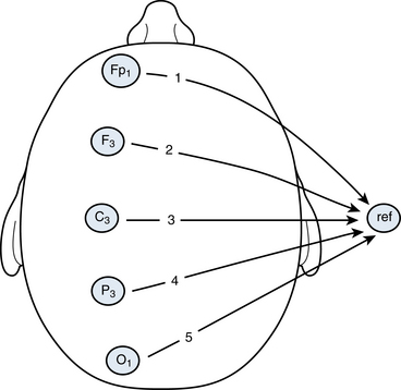
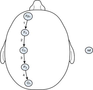
Figure 5-3 In this illustration, the same five parasagittal electrodes used in Figure 5-2 are connected to each other sequentially in a standard “bipolar chain.” Again, each arrow points from an Input 1 electrode to an Input 2 electrode creating the following montage: Fp1-F3, F3-F3, C3-P3, and P3-01. The reference position is not used. Each of the four channels generated with this technique represents the subtraction of an electrode from the previous electrode in the chain. Because the electrodes are paired to form each channel, five electrodes generate four channels of output.

Note that, even the so-called referential montage is, in reality, “bipolar.” Every channel must represent a comparison of two electrode positions—there are always two “poles” being compared. This is one of the criticisms of the term bipolar montage; it seems to imply that the counterpart term, referential montage, is not bipolar in some way. Indeed, there is no such thing as a “monopolar” montage, and technically all montages are, at their root, “bipolar” because every channel displayed on the EEG page, be it part of a bipolar or referential montage, is a voltage comparison between at least two points.

Theoretical Strategies: How Can EEG Activity Best Be Recorded From a Single Point?

It is useful to consider the theoretical pros and cons of each recording technique starting by asking the elemental question: what would be the best way to demonstrate the electrocerebral activity at any given point on the head? Consider the example of the left frontopolar area, where the Fp1 electrode records at a point on the forehead above the left eye. If we were assigned the task of deciding how best to record the electrical activity occurring under the Fp1 electrode, momentarily leaving aside what is going on elsewhere in the brain, what would be the best way to do this?

Recalling that our basic tool for creating an EEG channel is to print the amplified output of a voltmeter for which the needle sweeps one way or the other depending on the voltage difference between two points, there must always be two separate amplifier inputs, Input 1 and Input 2, to make a comparison. We decide to attach the “electrode of interest,” Fp1, to one pole of our voltmeter (Input 1), but what would be the most advantageous choice of electrode(s) to attach to Input 2, the comparison point? This comparison electrode is called the reference electrode, and serves as the reference point against which the electrode of interest is measured. As described in Chapter 4, the voltage measured from the reference will be subtracted from the voltage measured at Fp1, and the resulting difference is the output for the channel that we will label as Fp1-ref.

It is clear that the choice of the reference electrode could have as big an impact on the appearance of the resulting output trace as the Fp1 electrode. At first glance, the channel label “Fp1-ref” may seem to imply that its output represents the voltage at Fp1. Note, however, that the “active electrode,” Fp1, does not enjoy any privileged position by being attached to Input 1 as opposed to Input 2; the two voltages will simply be subtracted one from the other and displayed. For that reason, if the chosen reference electrode were the earlobe and there happened to be more electrical activity present in the earlobe than in Fp1, the output of an Fp1-earlobe channel would be dominated by the electrical activity in the earlobe—not the desired result. Clearly, the choice of the reference electrode in referential montages is important.

Choice of a Reference Electrode

Considering different possible locations to place the reference electrode, because we are looking for a location with a “neutral” voltage for comparison, one possible choice would be an electrical ground. Possible grounds include the grounding prong from a three-prong wall outlet or a metallic cold water pipe that runs into the ground. In reality, the choice of attaching Input 2 to an electrical ground is not feasible. The resulting tracing would be full of noise, and we would have little success in our goal of displaying the very low-voltage EEG activity coming from the Fp1 electrode for two reasons.

First, electrical grounds, particularly those in large buildings such as hospitals, are not really electrically neutral. A variety of electrical devices throughout the building are attached to the same ground, and these devices spill electrical noise into the ground. Therefore, an Fp1-ground channel could include a terrific amount of noise from all of these distant sources and the signal of interest, the microvolt-level electrical activity emanating from the brain from the region of the Fp1 electrode, could be overwhelmed by all of this electrical noise.

The second and perhaps less intuitive problem is that the Fp1 electrode itself has a large array of electrical activity in it, but not all of that activity is brain wave activity. In addition to the very low-voltage activity that emanates from the left frontal pole of the brain (the activity that we really want to see), there is also a large amount of ambient electrical noise at that scalp location. Some of this noise comes from the human body, including electrical activity given off by the frontalis muscle of the forehead, electrical activity from the heart (the electrocardiogram), electrical noise from movement of the eyes, and even noise from swallowing movements. Even more troublesome, however, is the fact that, especially indoors, the environments we live in are full of electrical activity. Relatively large amounts of electrical noise flow through our bodies at all times, especially in electrically active environments such as hospital rooms or EEG laboratories where EEG recordings are usually performed. As previously described, contamination of our bodies with 60-Hz signals from electrical outlets is especially common. Comparison of Fp1 to a completely indifferent electrode (such as an ideally quiet ground) would do nothing to attenuate (or “subtract out”) the large amount of electrical noise in the vicinity of the Fp1 electrode in favor of the true brain wave signal in that area. Therefore, paradoxically, we do want some noise in the reference electrode. Ideally, we would like the reference electrode to have the exact noise that is present in the Fp1 electrode so that our differential amplifiers will subtract it out.

Considering these goals, choice of an ideal reference electrode becomes an interesting challenge. Instead of using electrical ground as the reference electrode, consider the possibility of using an electrode placed on the foot. The choice of the foot electrode would be a vast improvement over using the ground because a recording electrode on the foot would detect a lot of the same electrical “body noise” as an electrode on the head (and also would lack the ground noise). Because the signals from Fp1 and the foot would be subtracted from one another, electrical noise in the body common to both locations would cancel out and only the difference would appear in the resulting tracing. The chance that the brain wave signal we seek under Fp1 would rise above the fray and be recognizable to us is now much higher.

Next, consider the idea of using an electrode position adjacent to Fp1 (such as Fp2, the electrode over the right frontal pole) as the reference electrode. Subtracting Fp2 from Fp1 yields a signal that appears much cleaner and will be of lower voltage compared with the Fp1-foot pairing. At first glance, this Fp1-Fp2 pairing would seem to be the most satisfactory because the amount of noise in the channel is minimized—any eletrical noise in Fp1 is probably also present in Fp2 and that common noise should cancel out. However, there is also a significant potential disadvantage that may not be obvious at first glance. If there is brain wave activity common to both the Fp1 and Fp2 electrodes, the subtraction of the Fp2 signal from Fp1 may actually cancel out some of that common brain wave activity, the activity we actually seek to record. The only signal displayed will be the difference between the two locations that may only represent a portion of the total brain wave activity at Fp1, the display of which was the original goal of picking an ideal reference. The idea that there could be a lot of brain wave activity in common between Fp1 and Fp2 is plausible because there could be, for example, a frontal slow wave shared more or less equally by Fp1 and Fp2. The common mode rejection amplifiers used in our EEG instruments would cancel some or all of this common brain wave activity when the Fp2 activity is subtracted from Fp1. We would then have a tracing that appears to be “electrically clean” at the expense of losing some of the EEG activity we are looking for.

Finally, consider the extreme example of moving the reference electrode so close to Fp1 that it is nearly in the same position as Fp1. In such an example, the signal in Fp1 and the reference are so similar that the difference output will become nearly flat. Some generalizations can then be made regarding the distance between the electrodes attached to Input 1 and Input 2 of a channel’s amplifier. When two electrodes are moved closer to one another, there is greater commonality between what each detects in terms of both the noise signal and the brain wave signal. Therefore, as two electrodes become closer to one another, a channel comparing them will flatten. Conversely, as interelectrode distances increase, there is a bigger difference in both the noise signal and the brain wave signal and the channel”s output signal tend to increase.

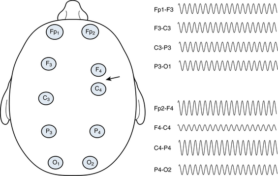
All things being equal, larger interelectrode distances are associated with higher voltages, and smaller interelectrode distances are associated with lower voltages. This effect explains the recommendation that electrodes should not be skipped in bipolar montage chains (or stated another way, that interelectrode distances should be held constant). A channel pair with an inconsistently large interelectrode distance will tend to produce a higher voltage channel, possibly giving the erroneous impression that there is more electrical activity at that location than at adjacent locations. Variation in interelectrode distances may occur in two ways: a montage design that skips an electrode or a significant mismeasurement of electrode position during electrode application (see Figure 5-4).

Figure 5-4 This figure illustrates the consequences of mismeasurement of electrode positions. Note that the electrodes of the left parasagittal chain, starting with Fp1, are measured in the usual way with constant interelectrode distances. The electrode positions of the right parasagittal chain, however, have been mismeasured so that the F4 and C4 electrodes have been placed too close together, resulting in an inadvertent increase in the interelectrode distance in the Fp2-F4 and C4-P4 electrode pairs, while the F4-C4 interelectrode distance is too small (arrow). The left parasagittal chain, the output of which is represented by the top four channels on the right side of the page, correctly displays equal voltages in each channel. As a consequence of the mismeasurement in the right parasagittal chain, the channels for which interelectrode distances are too large, Fp2-F4 and C4-P4, show exaggerated, higher voltages, and the channel with the decreased interelectrode distance, F4-C4, shows a misleadingly decreased voltage. Note that if each of these chains had been displayed using a referential montage, the error in measurement in the right parasagittal chain would not necessarily be evident.

What would the ideal reference electrode location be?

The ideal reference electrode includes all of the electrical noise in the “electrode of interest” but none of the electrocerebral activity.

It will come as no surprise that no such ideal reference electrode exists. The goal is to find some compromise location for the reference electrode that will tend to cancel out noise fairly well but will not cancel out too much brain wave activity. The choice of a good reference electrode position represents a balance between wanting the electrode to be close to the “electrode of interest” so that it will share as much noise signal with it as possible and wanting it to be distant enough so that there is not too much cerebral activity in common between the two electrodes (to avoid cancelling out EEG information). Commonly used reference points include the earlobes or mastoid areas, the nose, the CS2 location representing the skin overlying the spinous process of the seventh cervical vertebra (vertebra prominens or the most prominent bony bump at the base of the neck), or more rarely the Cz electrode. More complex reference electrodes may be used as well, including techniques in which the arithmetic mean of some or all of the scalp electrodes is used as a “virtual” reference electrode (discussed later in more detail). Each of these techniques is associated with its own advantages and disadvantages, which will also vary according to clinical circumstance.

Each potential reference location is prone to certain problems and advantages—no single reference electrode position is ideal for all patients at all times. For instance, the earlobes often share a portion of the electrocerebral activity present in the adjacent midtemporal areas, causing a cancellation effect. This makes an earlobe reference a poor choice for a patient with a high voltage midtemporal discharge. Also, the left earlobe in particular is often contaminated with EKG artifact because of the left-sided position of the heart. In some, the nose reference may be contaminated by a surprising amount of muscle artifact, whereas in others it can be fairly clean. The cervical area is contaminated by muscle artifact or EKG signal in some patients and may also be disturbed by movement when patients are lying on their backs. The midline vertex electrode, Cz, is usually free of muscle artifact because of its location at the vertex of the scalp but contains a large amount of electrocerebral activity, especially during sleep. In different individuals, any of these reference locations could generate satisfactory or unsatisfactory recordings at different times.

In the case of designing a referential montage, after the reference electrode has been chosen, there is little more to decide than the order to arrange the channels on the page. There are two general strategies for channel arrangement. One is to arrange the channels in left–right pairs so that each position on the brain can be compared with its homologous counterpart in the opposite hemisphere. This approach leads to a “left–right–left–right. . .” arrangement of channels (e.g. Fp1 followed by Fp2, F7 followed by F8, F3 followed by F4, and so on). The alternative strategy for ordering the channels conforms to the “left-over-right” and “front-to-back” conventions mentioned above in which channels are “clumped” according to their location. Although each of the two systems offers specific advantages, neither is clearly superior to the other as each EEG electrode’s channel will appear somewhere on the page with either system, only in a different order.

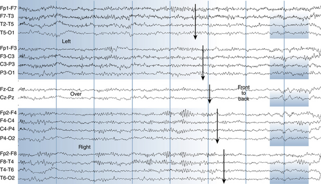
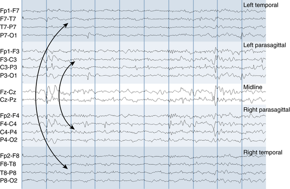
The main difference between the two systems, one of which alternates left- and right-sided electrodes and the other of which groups left-sided electrodes in one area and right-sided electrodes in another, is the comparative ease of visual scanning for asymmetries. Choice of one of these arrangements over the other is essentially a matter of preference. Figures 5-5 and 5-6 show examples of dramatic left-sided slowing displayed with each of these two common strategies. The latter system, which groups electrodes together by location, is seen to have certain advantages. Asymmetries that occur between hemispheres are not usually localized to a single electrode but to a regional group of electrodes. For instance, if a temporal slow wave is present, it may be recorded in multiple electrodes such as F7, T7, and P7. When an abnormality such as a spike or a slow wave is present in multiple adjacent channels on a page, it tends to be easier to identify visually when the spatial clustering system is used. In the alternating left–right setup, the abnormality will only be seen in alternating channels. Another advantage of the clustering system is the ease of visualizing the topography of the discharge on the scalp; with this system a region of the page corresponds to a region of the brain starting with the fact that the left hemisphere is represented on the top of the page and the right hemisphere is on the bottom. Grouping the channels by region, especially when gaps are used between electrode groups as in the example illustrated here, makes it simple to know where a given channel is on the head at a glance, even without reading the channel labels. In contrast, when reading in a montage in which the left and right channels are alternated, it can be difficult to know the location of each electrode without consulting the channel labels. Proponents of the left–right alternating system like the fact that homologous channels are adjacent to one another, making individual interchannel comparisons easier. Considering these reasons together, the author prefers the clustering system (left over right and front to back), which should allow for easier and more accurate scanning and spatial visualization for most readers. However, the choice of either of these two arrangements is really a matter of laboratory or reader preference.

Figure 5-5 This EEG page shows an example of left hemispheric delta activity shown in a referential montage in which the channels are ordered on an alternating left–right basis. This commonly used arrangement has the advantage of allowing the reader to compare homologous areas of the brain in adjacent channels. For instance, the top two lines show channels comparing the left frontopolar area to the right frontopolar area, and so on. In this case, the reference used is an average of the A1 and A2 electrodes (placed on the left and right earlobes, respectively). Close observation reveals, at least on the top half of the page (and therefore over the anterior portion of the brain), that every other channel shows a more prominent delta wave, indicating increased slow wave activity over the left anterior hemisphere.

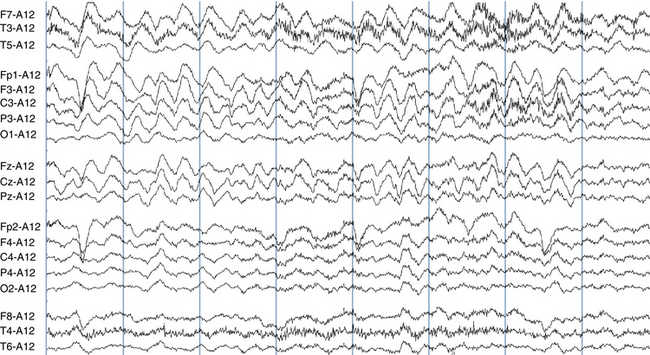
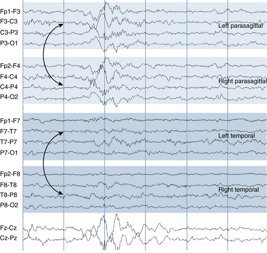
Figure 5-6 This EEG page shows the exact same left-sided slowing as was seen in the previous figure, however, the channels are ordered in chains so that the left hemisphere electrodes are shown on the top half of the page and the right hemisphere electrodes on the bottom. Starting at the top, channels are grouped on the page as the left temporal, left parasagittal, midline, right parasagittal, and right temporal chains (see channel labels). The same reference is used as in the previous figure, an average of the A1 and A2 electrodes. Note that, with nearby electrodes grouped together, it is visually much easier to appreciate the localization of the slowing over the left side of the brain (top half of the page). For this reason, this arrangement is favored by the author.

Bipolar Montages

In practice, most electroencephalographers do the bulk of their EEG interpretation using bipolar montages rather than referential montages, despite the potential disadvantages of the former. Bipolar montages are generally preferred because they produce “cleaner” tracings due to the proximity of the electrode pairs, which leads to more efficient noise cancellation. The clean appearance of the tracings and ease of reading does come at a potential price, however: the risk that the proximity of the electrode pairs has led to cancellation or an understated appearance of some of the brain wave activity, perhaps unbeknownst to the reader. When recording in a referential montage, if noise is present in the reference electrode, that noise may potentially obliterate all the channels at once. Given the different strengths and weaknesses of each technique, it is best practice to interpret any given EEG study using some combination of the two techniques.

Categories of Bipolar Montages

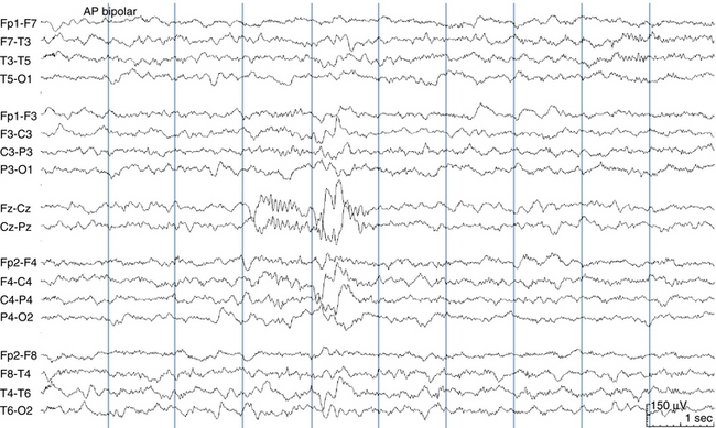
There are two principal categories of bipolar montages, the anteroposterior (AP) bipolar montage and the transverse bipolar montage. The two types differ in that, with AP bipolar montages, electrode chains run from front to back (anteroposteriorly) down the head, and in transverse bipolar montages, the chains run from left to right (transversely) across the head. The fact that the reader has both of these montage families available for use raises the question of whether any particular discharge might only be visible in the AP bipolar but not in the transverse bipolar montage, or vice versa. Is it really necessary to use both AP and transverse bipolar montages for EEG interpretation, and, if so, what would be lost by not doing so?

It is true that the large majority of discharges seen in an AP bipolar montage will also be visible in a transverse bipolar montage; however, there are exceptions. Certain discharges may show a steep gradient in the AP direction and a shallow gradient in the transverse direction (or vice versa). Although such discharge topographies are relatively infrequent, examples of scalp events that are only evident in one type of bipolar montage but not the other do occur.

Using a combination of these two montage types may also aid significantly in localization. The AP bipolar montage will indicate the maximum of the discharge in the front-to-back direction, usually by the location of a phase reversal. Likewise, the transverse montage will localize the maximum of the discharge in the left-to-right direction. Combining the two techniques allows localization of the maximum on a two-dimensional model of the scalp surface.

Circumferential Montages

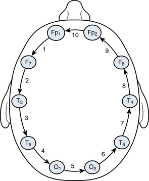
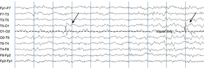
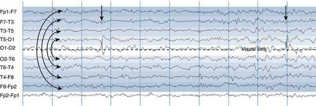
Some laboratories also use a third ordering for bipolar electrode chains, one that makes a complete circumference around the head (see Figure 5-7). This style of montage has been given a variety of names, such as a halo, circumferential, or hatband montage. Close examination of the electrode pairs used in the circumferential montages shows that almost every pairing is also present in the standard AP bipolar montage. The only electrode pairings that are unique to circumferential compared with AP bipolar montages are the Fp1-Fp2 and O1-O2 pairs. Because these two pairs are included in the transverse bipolar montages, circumferential montages are not a mandatory member of a laboratory montage set, although the decision to use such a montage is at the discretion of the electroencephalographer. For this reason, the use of a minimum of three montages—AP bipolar, transverse bipolar, and referential—is usually adequate to cover all necessary electrode pairings in standard EEG recording. Circumferential montages, when used, lend themselves to a particular technique for visual scanning. A visual axis is chosen and surrounding channel “layers” are compared (see Figures 5-8 and 5-9).

Figure 5-7 This arrangement of a bipolar chain that encircles the head is called a circumferential, halo, or hatband montage in different laboratories. In the arrangement shown in this figure, the electrode chain starts with Fp1 and proceeds in a counterclockwise direction. In some versions of this montage, the circumferential chain can start with one of the occipital electrodes.

Figure 5-8 A circumferential bipolar chain is shown. Note the spike-wave discharges (arrows) phase-reversing in the O1 electrode. It is clear that the discharge represents an asymmetrical event because it is confined to one side of the visual axis, which is represented by a dashed line.

Figure 5-9 The same page of EEG material from the previous figure is shown with arrows and shading that suggest a method for visual scanning of a circumferential montage. Comparisons are made about the inner (white) channel with the dashed line, which represents the “visual axis.” Like-shaded areas represent homologous areas of the brain. For instance, higher voltage slowing in one dark blue band compared with its counterpart on the opposite side would suggest an asymmetry of that slow activity between the hemispheres.

Disadvantages of the Bipolar (Differential) Technique

We have already alluded to certain disadvantages of the bipolar montage strategy. These stem from the fact that we are looking at the display of the differences between electrodes that are quite near and, typically, adjacent to one another. Clearly, a significant amount of information can be lost using this technique. An analogy for how information is lost with the bipolar technique is illustrated by the following example: imagine that we are told about the weather during a 5-day period in the following fashion: “Between Monday and Tuesday, it got five degrees warmer, and on Wednesday it got another three degrees warmer. By Thursday the temperature dropped seven degrees, and by Friday the temperature dropped another two degrees.” Although there may be a lot of accurate information in these two sentences, the reader still cannot tell whether it is hot or cold outside. All of the information is given as subtractions, the difference between one day’s temperature and the next. We don’t know whether the temperature was below zero throughout this time period or whether these facts describe the temperature changes during a very hot week in July. All we know are the relative ups and downs. Likewise, in a bipolar montage, when we note pen deflections telling us that voltages are getting more negative or more positive as we travel along a chain, we do not get absolute voltage information.

At first glance, if the bipolar montage recording system were as poor as the temperature reporting system given in this example in which we could not tell a hot day from a cold day, how is it that bipolar montages are useful at all? The answer is that, when we read an EEG page, we make an implicit assumption that the average baseline of everything that we see printed out is near neutral voltage (or “zero”). Indeed, because of the laws of electricity and charge, it is quite unlikely that all scalp areas will be either strongly negative or strongly positive for a prolonged period of time. Therefore, as we read, we are making a subconscious assumption that the average of everything that we see on the page is near zero. Nevertheless, we do lose absolute voltage information. We cannot know whether certain events may be slightly positive or slightly negative just by looking at the bipolar montage; we can only assert that an event is, for instance, “more negative” than the areas around it. For this reason, absolute measurements of voltage cannot be made as easily as they can be in a referential montage or, if they are made, they mean something different. When a reference electrode is used, we are making the implicit assumption for the purposes of measurement that the voltage at that electrode is neutral or zero (although we might shy away from making this assumption at a time that there is clearly a lot of noise in the reference electrode). This assumption is shakier when made in a bipolar montage, a system in which we only see voltage differences between nearby points on the scalp rather than absolute voltage measurements.

An extension of the problem of not knowing the absolute magnitude of the voltage at any given point when reading in a bipolar montage is the tendency for cancellation of like activity in adjacent electrodes. Here, again, we can imagine a case in which there is a posterior slow wave more or less equally represented in the three posterior electrodes: C3, P3, and O1. In such an example, when recording with a bipolar montage, this posterior slow wave could cancel itself out to a large extent in the areas where it is at highest voltage, simply because it happens to be equally represented between the pairs of electrodes being compared (e.g., C3-P3 and P3-O1). This effect is illustrated in Figure 5-10. This effect does not occur in referential montages.

Figure 5-10 (A) EEG activity displayed in a referential montage and (B) shows the exact same activity displayed in a bipolar montage. Panel A shows fairly prominent alpha activity, especially in the three posterior channels (C3, P3, and O1) during the first (arrow) and third seconds. Note that this posterior-predominant alpha activity is relatively difficult to see in Panel B when the subtractions for the bipolar montage take place. The mathematical reason for this becomes evident when analyzing the alpha waves shown at the upper point of the double-headed arrow. Because the phase and shape of these waves are seen to be quite similar in the C3, P3, and O1 channels in the referential montage (Panel A) there is significant cancellation in the bipolar display shown (Panel B). In fact, these waves can barely be recognized in the P3-O1 channel, even though they are strongly present in both P3 and O1. Because of effects such as these, it is preferable to confirm subtle voltage asymmetries seen in bipolar montages by checking a referential montage.

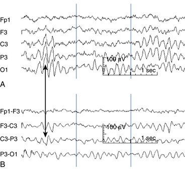
This is one of the main disadvantages of bipolar recordings—that adjacent, in-phase activity tends to cancel out. This can cause a paradoxical effect: disappearance of a wave in an area where its voltage is highest and appearance of that wave only when a chain moves into an area where it begins to disappear. It is in the comparison of the area where the wave is present to the area where it disappears that the “difference” is picked up by the bipolar recording technique, not necessarily the area in which the voltage is highest. Some of these effects are also illustrated in the exercises in Chapter 4 on localization. Fortunately, in practice this effect is not as big a problem as it might seem to be, because like activity in adjacent electrodes is often out of phase (not perfectly lined up with the wave in the adjacent electrode) and therefore does appear in the “correct” location in bipolar montages after subtraction. Still, it is wise to confirm a mild voltage asymmetry noted in a bipolar montage by reexamining it in a referential montage to exclude this potential shortcoming of bipolar recordings.

Techniques for Visual Scanning of Montages

AP Bipolar Montages

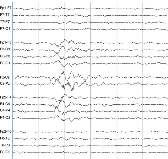
After you are familiar with the montage set used by your laboratory, it is useful to develop a visual scanning strategy for each montage in the set, a visual method or thought process for looking at each page of EEG that allows quick determination of interhemispheric or anterior versus posterior asymmetries. The first example we will look at is the standard AP bipolar montage used most frequently in the examples in this book. This AP bipolar montage conforms to the conventions suggested by the American Clinical Neurophysiology Society (ACNS) in that it uses the left-over-right and front-to-back conventions. Figure 5-11 uses shading to demonstrate the technique for detecting asymmetries. An axis should be imagined through the two midline channels, which have been left unshaded and represent the cranial midline. Next, the two inner (parasagittal) chains, which are lightly shaded in blue, should be compared. Is there more slow activity or fast activity in one light blue area compared with the other light blue area? If so, a parasagittal asymmetry is likely. Similarly, is there an asymmetry of activity between the more darkly shaded outer (temporal) chains? If so, a temporal asymmetry may be present.

Figure 5-11 This schematic shows the visual scanning strategy used to compare homologous areas of the brain for the standard anteroposterior bipolar montage most commonly used in this text. The anteroposterior chain groupings progress from left to right as the eye scans down the page. The outer channel groups, shaded darker blue, represent the temporal areas and the inner channel groups, shaded lighter gray, represent the parasagittal areas. The unshaded strip of two channels in the middle of the page corresponds to the midline of the head. Note that the sleep vertex waves in the second and eighth seconds manifest as bursts of sharp waves seen fairly symmetrically in both parasagittal areas and in the midline but do not involve the temporal chains, as expected for vertex waves of sleep. By contrast, nonsymmetrical scattered spikes are seen in other locations. Identify the low voltage spikes at C3, O1, and C4.

Other laboratories may use the left parasagittal/right parasagittal/left temporal/right temporal ordering for the AP bipolar electrode chains. If so, the scanning strategy is adjusted accordingly. Figures 5-12 and 5-13 show a comparison of the two most common arrangements for the AP bipolar montage. Neither is technically superior to the other because both include the exact same set of channels, simply presented in a different order, and each will be commonly encountered in different laboratories.

Figure 5-12 An example of vertex waves of sleep and sleep spindles is shown in the standard anteroposterior bipolar montage most commonly used in this text. The reader should appreciate that the topography of the page going from top to bottom corresponds to a left-to-right sweep across the head, as if from left ear to right ear. A main advantage of this system is that chains that are adjacent on the head are adjacent on the page.

Figure 5-13 The same page of EEG as in the previous figure is shown in an anteroposterior bipolar montage using another common ordering of the chains. The shading and arrows imply visual comparisons of homologous areas. The top two sets of four channels correspond to the left and right parasagittal areas, and the bottom two sets of channels, shaded darker blue, correspond to the left and right temporal chains. In this setup, the midline channels are at the bottom of the page. This system may facilitate comparison of like areas but requires the eye to jump around the page more to localize events because topographically adjacent areas are no longer adjacent on the page.

Transverse Bipolar Montages

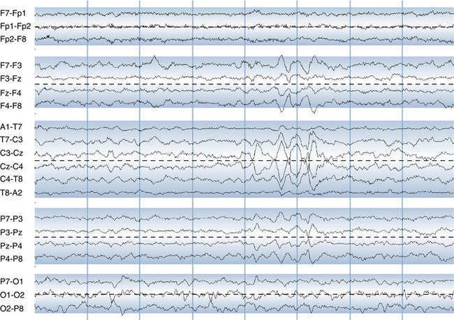
The transverse bipolar montage can be scanned in a fashion that is somewhat similar. Again, note the shading of each group shown in Figure 5-14. In this text, most illustrations of the transverse bipolar montage include a white space (a “gap”) inserted between each chain, making it visually simpler to scan, although the practice of inserting these gaps is not common to all laboratories. Gaps make it easier to see the groupings of individual electrode chains, but they sacrifice space on the page and therefore diminish the amount of line height that can be assigned to display each channel. The dashed lines in the figure suggests the axis around which each electrode chain should be visually scanned. If channels look different in the area above the axis compared with the area below it, this suggests a difference in that chain between the left and the right sides of the brain. The reader should practice visualizing the superimposition of this shading on the page to help quickly determine which part of the page corresponds to which part of the brain.

Figure 5-14 The figure shows an example of Stage II sleep displayed in a transverse bipolar montage. Each of the six chains is shown with gradient shading denoting the distance of each channel from the central visual axes, which are indicated by the dashed lines. In each grouping of channels, areas of like shading are compared with one another to establish symmetry. An event occurring above the visual axis but not below the axis in a group, be it a slow wave or a sharp discharge, suggests an asymmetry of that event between the hemispheres.

Montages for Special Situations

The montage setups just described represent strategies useful for standard situations. When a patient has a surgical incision or some other obstruction to electrode placement, the technologist must often decide how to rework a montage “on the fly” to make a useful display of the data despite the unavailability of certain electrodes. Standard montages must also be modified when additional electrodes are used. When doing so, keeping interelectrode distances consistent, if possible, can eliminate the effect of a channel manifesting a higher voltage simply because of increased interelectrode distance. In some situations, though, variation of interelectrode distances may be unavoidable. The question of whether a voltage change is the result of a variation in interelectrode distance can usually be resolved by analyzing referential montages which are not sensitive to variations in interelectrode distance.

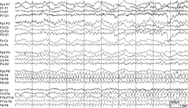
Regarding the use of additional electrodes, the most common “extra” locations added are the T1 and T2 electrode positions, which are designed to record from the anterior temporal lobe. The T1 and T2 names represent old nomenclature and correspond approximately to the FT9 and FT10 electrode positions of the modified 10-10 electrode system. A variety of methods can be used to incorporate these additional electrodes into a display montage. An example montage is shown in Figure 5-15. Use of these special temporal electrodes has to a great extent supplanted the use of more invasive electrodes, such as sphenoidal and pharyngeal electrodes.

Figure 5-15 This EEG page shows an actual electrographic seizure discharge recorded with additional FT9 and FT10 electrodes (similar in position to the T1 and T2 electrodes used in other laboratories). The top 18 channels are identical to the standard anteroposterior bipolar montage used elsewhere in this text. The bottom five channels consist of a loop that includes the additional temporal electrodes. This seizure discharge is initially picked up well by electrodes at T8, P8, and FT10, as well as other nearby electrodes. The loop of five electrodes at the bottom of the page can be visually scanned imagining a visual axis through the middle FT9-FT10 channel. Note in this case that the seizure discharge begins below the axis defined by the FT9-FT10 channel (beginning of the page) implying that it has started on the right side of the brain. By the end of the page, the discharge is seen both above and below the axis, implying that it has become bilateral.

The Choice of the Reference Electrode (Revisited): “More Important Than It Seems”

As described earlier, the choice of the reference electrode can have a large impact on the appearance of the resulting EEG tracing. Recall that, when looking at a channel labeled Fp1–reference (abbreviated as Fp1–ref in this text), there is an implicit suggestion that the signal we are seeing represents activity from Fp1. In the best of all possible worlds, this is true (because in the best of all possible worlds, the reference electrode is completely indifferent or neutral). It is worth keeping in mind, however, that the “electrode of interest,” Fp1, and the reference electrode have the same potential to contribute to the appearance of the final output; neither has “mathematical” primacy over the other. The Fp1–ref channel only successfully represents Fp1 activity when the reference is quiet. Under what circumstances is the reference not quiet, and how might this affect our choice of reference for any given patient at any given time?

The importance of being aware of what reference electrode is in use at any given time when interpreting a referential montage cannot be overstated. There are several reasons for this, but two are particularly important. First, if there is noise in the reference electrode, that noise will appear in every channel in which that reference electrode has been used. Remembering that the reference electrode has as much potential to affect the tracing as the “electrode of interest,” whatever noise appears in the reference will likely appear in the output signal. Because different reference electrodes are more likely to generate specific types of artifact, knowing which reference electrode is in use helps the reader correctly reject certain waveforms as artifact. Therefore, if a wave is seen in a channel, the reader must ask whether it comes from the electrode of interest or from the reference electrode. This thought process must be used for all waves of significance identified in the EEG when referential montages are used.

The second, more complex type of problem arises when the reference electrode itself is picking up brain wave activity. A commonly used reference, the earlobe, is well known to pick up a portion of temporal lobe activity in many patients. What impact might this fact have on the display of a temporal lobe discharge when an earlobe reference is used? As you may have guessed, when the reference electrode is “active” with a discharge, it will tend to cancel that discharge in the temporal lobe channels when the subtractions take place; the resulting display will appear to understate the voltage of the discharge. In the most extreme example, if the discharge is picked up equally well by the earlobe reference and T7, the discharge could conceivably be completely cancelled out in a T7-earlobe channel.

There are three scenarios to consider in the undesirable situation in which the reference electrode picks up an active discharge. In the first, the “electrode of interest” is recording a discharge and is being compared with a reference electrode that is also recording the discharge (at least partially). In the second, the “electrode of interest” is in an electrically quiet area (such as the right occipital area in the above example), but the reference electrode (the earlobe) is picking up a portion of the discharge. In the third there is some other type of electrical noise contaminating the reference electrode. Each of these possibilities is discussed below.

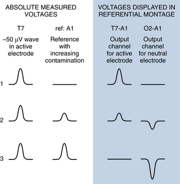
Figure 5-16 shows examples of the first two situations and illustrates the effects of increasing spillover or contamination of the reference electrode (in this case, the left earlobe) of a discharge picked up by T7 (the left midtemporal electrode). It also shows the potential pitfalls of using the earlobe reference to display the activity at a distant, inactive location such as O2 (the right occipital electrode) when there is contamination of the reference. Because the discharge does not involve O2, the reader would expect that the O2 channel will be flat, but this is not the case when an earlobe reference (A1) that is contaminated with an active discharge is used in a channel (O2-A1) to display O2 activity. This is a realistic example because the ipsilateral earlobe often does have brain wave activity in common with the left midtemporal area. An example of a third type of situation in which unrelated noise contaminates the reference electrode is shown in Figure 5-17.

Figure 5-16 This figure illustrates how increasing amounts of contamination of the reference electrode (A1, or the left earlobe, in this example) affect the appearance of the output channels for both an electrode that is “active” with a discharge (T7 or the left midtemporal electrode in this example) and for a theoretically neutral electrode (O2 or the right occipital electrode in this example). The examples shown on rows 1, 2, and 3 all assume a sharp wave discharge of the same strength in T7 (depicted in the first column) however, the amount of the discharge picked up by the A1 reference electrode (the amount of “contamination” of A1) increases in each row (depicted in the second column). By the bottom row, the amount of the T7 discharge that spills over into A1 begins to match the voltage picked up by the active electrode, T7. The first two (unshaded) columns show the “true” amount of voltage change present in the T7 and A1 electrodes; the O2 electrode is assumed to be neutral. The second two (shaded) columns show the appearance of the output channels for T7-A1 and for the distant and inactive right occipital area, O2-A1 as they would appear on the EEG screen. Each channel output is based on the subtraction of the voltage of the second electrode in the pair from the first, as usual.

Row 1 shows the simple case in which T7 is active and the A1 reference is neutral or “clean.” In this case, the T7-A1 channel shows an accurate representation of the activity at T7. There is no problem in the O2-A1 channel; O2 is quiet and the A1 reference is clean, so the O2-A1 channel accurately portrays the lack of activity at O2. In Row 2, the activity at T7 is unchanged, but now the A1 reference picks up some 50% of the T7 discharge. Now the T7-A1 channel will display the discharge, but only at one half its actual height. Worse, however, is the fact that a “flipped” version of the discharge is seen at O2-A1, even though O2 is an area that we know to be electrically inactive. Finally, we consider the example of Row 3 in which the A1 reference electrode picks up the discharge just as well as the “active” T7 electrode. The channel outputs are now quite misleading; the discharge is absent from the T7-A1 channel (even though we know this to be a T7 discharge), and now the O2-A1 channel, which is presumably representing the activity in the quiet right occipital area, has a large (but “flipped”) discharge because of the contaminated A1 reference. A combination of a careful eye and review of other montages (including bipolar montages) may be necessary in order not to be led astray when real-life EEG discharges resemble the examples shown in Rows 2 and 3.

Figure 5-17 This EEG page is displayed in a referential montage with the nose used as the reference. When there is electrical noise in the reference, it will appear in every channel in a more or less identical fashion. The light gray arrow shows a single, low-voltage transient, the origin of which is likely the nose. Note that this transient manifests the same shape and has similar polarity and voltage in all channels. Likewise, a burst of muscle artifact is seen in all channels one second later (dark arrow), also likely of nose origin because of similar morphology in all channels. The higher voltage of muscle artifact in the T8 channel probably represents a mixture of muscle activity in the nose and additional muscle activity from the T8 (right midtemporal) area.

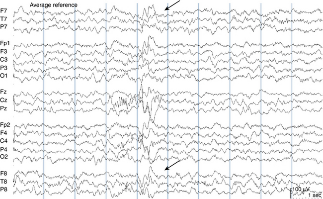
The Average Reference: Strengths and Weaknesses

The “average reference” montage is a favorite among some electroencephalographers but disliked by others. In practice, montages that use the average reference are neither “good” nor “bad”; in some circumstances they are very useful, whereas in others their disadvantages are so substantial that they can lead to serious reading errors and should not be used. The average reference is a simple arithmetic average of all the electrodes on the scalp chosen to be in the average. As expected, it can be calculated by summing the voltages measured by all of the electrodes used and dividing by the number of electrodes. Although the average reference can be defined to use all of the scalp electrodes, sometimes certain noisy electrodes may be excluded from the average, such as Fp1 and Fp2, which are often contaminated by high voltage eyeblink artifact.

When considering the possible value of the average reference, the first impression may be that the average reference represents brain activity and that perhaps it is a bad idea to subtract brain activity away from the signal being displayed. The counterargument to this is that the brain activity in all scalp electrodes, when averaged, should tend to self-cancel leaving a relatively “clean” average that is near zero. This condition does hold much of the time but, as we shall see, not all of the time. Another potential strength of the average reference is seen when an identical noise signal is present in all electrodes, a situation that is not uncommon. In such cases, that signal will remain represented in the average reference and be available to cancel out that same noise signal in the “electrode of interest.” For example, a 20-μV “spike” of noise contaminates every scalp electrode; it will then average to 20 μV in the average reference and is subtracted from every electrode of interest in an average reference montage effectively removing the spike. When will each of these conditions hold true, and when will they not?

When reading an EEG tracing in an average reference montage, a good strategy is to estimate what the average reference signal should look like at any moment. Considering all the channels together, the average reference can be visually estimated by mentally summing up the voltages of all the channels, noting the relative strength of upgoing waves compared with downgoing waves and predicting the average. It is clear that when the various channels are of low voltage and there is not much activity, the average reference, too, will be of low voltage and relatively neutral. At such times, the average reference generally gives a very clean and useful comparison. What happens, though, when there is a lot of activity in the EEG? In the case of a very focal spike, when it is averaged among the large number of inactive electrodes, that spike’s voltage becomes diluted significantly when averaged with the quiet electrodes and may have little visible effect on the average. What if the spike is present in several electrodes, or what if the spike is of particularly high voltage? As an electrical scalp event rises in voltage or is present in an increasing number of electrodes, it will clearly affect the average reference to an increasing degree. When discharges on the scalp make the average reference “active,” it is important to remember that this activity will now be subtracted from every “electrode of interest” in the montage.

Consider the simple example of a 20-electrode set, and, at one point, the reader notes that two of the channels measure −100 μV and the other 18 channels are flat (0 μV). The value of the average reference electrode at that time will be (−100 + −100) / 20 or −10 μV. The two electrodes that are active with the −100 μV spike will be compared with the −10 μV reference (−100 μV minus −10 μV = −90 μV) and display a −90 μV (upward) deflection, which is a satisfactory approximation of the true −100 μV spike. The same subtraction also takes place, though, for each of the inactive electrodes so that any inactive electrode’s channel when compared with this average reference will show a small positive (downward) deflection of 10 μV, even though these electrodes are, in reality, neutral (Input 1 electrode equals zero and Input 2 electrode equals −10; Input 1 − Input 2 = +10 μV). This small amount of deflection may be tolerable, especially if it is expected by the alert reader who predicts that the average reference will be mildly negative at that moment on the basis of observation of all of the channels. A reader who does not take this effect into account could erroneously conclude that there is a low-voltage concurrent positive spike occurring broadly across the brain, which is not the case.

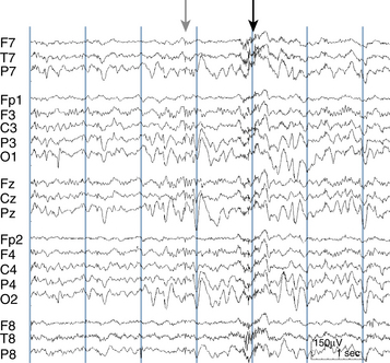
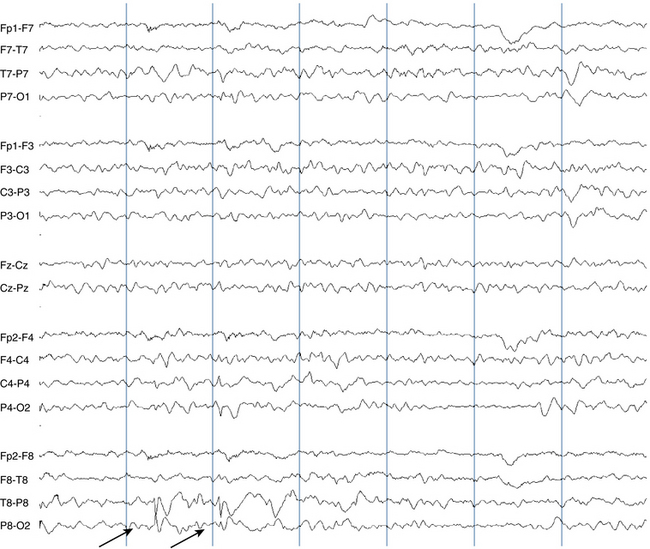
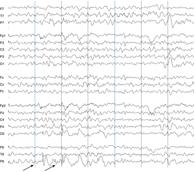
Figures 5-18 and 5-19 show an example of an effective use of the average reference. In this example, a spike in P8 is so focal that it does not contaminate the average reference to any significant extent and the average reference montage displays an excellent representation of the field of the spike. Figure 5-20 shows an example of a seizure discharge with a broad field across the right hemisphere that is clearly restricted to the right side of the brain, displayed in a bipolar montage. Considering what this discharge might look like if displayed in an average reference montage, the alert reader will note that the discharge involves many electrodes and would thus be expected to be visible in the average reference. Figure 5-21 shows the same page displayed in an average reference montage. Because the average reference is contaminated with the discharge, as expected, this montage gives the false impression that the seizure discharge is present on both sides of the brain.

Figure 5-18 Two spike-wave discharges are seen phase-reversing in the bottom two channels (arrows). The technique of identifying the location of the phase reversal efficiently identifies the point of maximum of this discharge as P8, the electrode shared by the bottom two channels (T8-P8 and P8-O2). Because the waves’ phases point toward each other, the spikes’ phase reversal indicates a negative spike. A comparison to the appearance of the same discharge displayed in a referential montage is shown in the next figure.

Figure 5-19 The same P8 discharges (arrows) from the previous figure are shown, this time in a referential montage in which the average reference is used. The localization technique for referential montages is used in which the maximum wave height, and therefore the discharge’s maximum, is identified at P8, the bottom channel. Because the spikes are upgoing we can conclude that the spike is negative with respect to the reference. Because the discharge is so focal and not of particularly high voltage, it does not significantly affect the average of all the electrodes. Therefore, in this case, the average reference is a satisfactory choice of reference to display this discharge.

Figure 5-20 This figure shows a low-voltage, repetitive seizure discharge with maximum in the right mid- to posterior temporal area (black arrow). The field of the discharge spreads to include the right parasagittal area (gray arrow). Note that the discharge is not present in the left hemisphere (the top eight channels), however. Some high-voltage artifact can be seen arising from the F7 electrode (asterisks) related to a poor contact, seen in the top two channels and unrelated to the seizure discharge.

Figure 5-21 The same right posterior quadrant seizure discharge as shown in the previous figure is now displayed in a referential montage using the average reference. Because the discharge involves several channels, when all scalp electrodes are averaged, the discharge is actually noticeable in the average reference itself. Note that, even though the discharge is well seen in the channels in which we know it to be maximal, T8 and P8 (black arrow), and also to a lesser extent in the right parasagittal chain, the discharge now falsely localizes to areas in the opposite hemisphere, even the left temporal chain where we know it not to be present (gray arrow). This occurs because the contaminated average reference is being subtracted from the electrodes in the inactive left temporal chain. A clue to the presence of this phenomenon is the “flipped” phase of the apparent seizure discharge in the left hemisphere. A reader who does not realize that the average reference is in use and contaminated by the discharge could erroneously report that this seizure discharge involves both hemispheres of the brain.

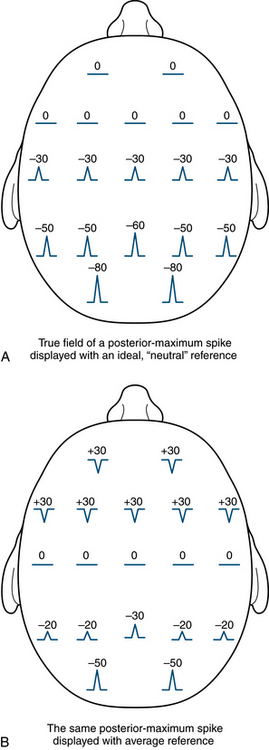
A schematic of an idealized posterior-maximum spike is shown along with numerical voltages in Figure 5-22 to illustrate the mathematics behind contamination of the average reference. The top half of the figure shows the “true” discharge, and the bottom half shows what the display will look like if an average reference montage is used. A reader who only sees the bottom display and who does not understand average reference montages may not appreciate that the discharge represents a simple negative spike involving only the posterior half of the brain.

Figure 5-22 The top panel (A) illustrates the true field of a spike discharge that is maximal in the occipital area with a field spreading forward to involve the posterior half of the head. The discharge does not, however, involve the anterior two rows of electrodes, which are shown in the diagram to measure zero voltage. The voltage measured at each electrode is given in microvolts. The bottom panel (B) shows the exact same spike, now displayed using an average reference. The resulting display can be predicted first by calculating the mean of the 19 recorded scalp electrodes, which comes to −30 μV (add all of the voltages in Panel A together and divide by 19), giving the voltage of the average reference. Because the average reference is attached to Input 2 of the CMR amplifier, its value will be subtracted from that of each Input 1 electrode. Arithmetically, the subtraction of −30 μV from each measurement is the equivalent of adding 30 μV (x − −30 μV is the same as x + 30 μV). Because of the convention of “pen-down = positive,” this subtraction results in each waveform being “lowered” by a height of 30 μV. Therefore, use of the average reference gives the unwanted effect of a broad apparent positivity in the neutral anterior electrodes (0 μV − −30 μV = +30 μV). It attenuates the apparent amplitude of the middle row of electrodes so that they appear neutral as shown and also attenuates the values of the more strongly negative electrodes in the posterior two rows. The alert reader must notice the unexpected “flipping” of the phase of the waveform between the front and the back of the head and consider the possibility that this atypical appearance may be related to a contaminated average reference rather than a discharge that is positive anteriorly and negative posteriorly.

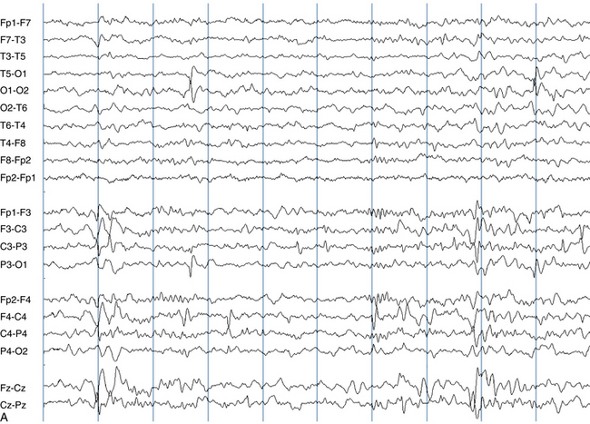
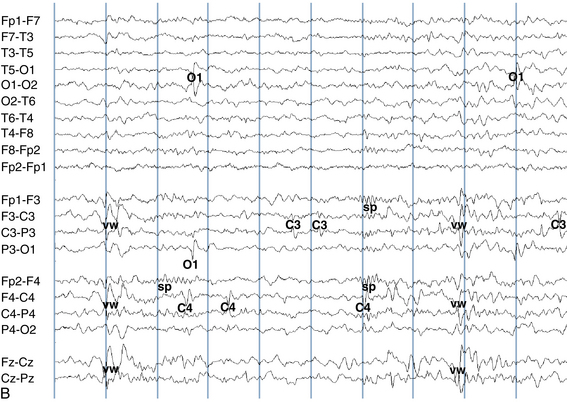
The average reference can be contaminated by nearly any type of EEG activity, not just by abnormal discharges. In some patients, normal activity such as vertex waves of sleep and sleep spindles are of high enough voltage and have a broad enough field they will affect all channels of an average reference montage, clearly an undesirable effect. Figures 5-23 and 5-24 show how even normal sleep activity can make a montage that uses the average reference confusing to interpret. Figure 5-25 shows the same page of EEG in an AP bipolar montage for comparison. The montage that uses the nose reference clearly shows the vertex waves and spindles in their proper locations, the midline and parasagittal areas; these waves are much less evident in the temporal chains. Because the spindles and vertex waves are widespread enough to contaminate the average reference, the average reference montage gives the mistaken impression that the field of the spindles and vertex waves extends strongly into the temporal areas, which it does not.

Figure 5-23 A page of EEG is displayed in a referential montage using the nose as the reference electrode. Stage II sleep is seen with vertex waves and spindles. Because the comparison electrode, the nose, represents a distant and indifferent reference point, this page gives an excellent representation of the field of both the spindles and vertex waves. As expected, the spindles are maximum in the central midline electrode, Cz, and also in the adjacent central C3 and C4 electrodes (arrows). The spindle field also extends forward to include F3 and F4. Likewise, the vertex waves seen in the following second have a similar field, maximum in the midline and in the parasagittal chains, but their field does not extend to the temporal chains to any great extent. Compare to the next figure.

Figure 5-24 The same page of the EEG as shown in the previous figure is now displayed using an average reference montage. Although the spindles are still seen to be maximum in Cz, they now appear to have a much broader field and are even seen in the temporal chains. The reason for this misleading appearance is that the average reference is “contaminated” with the spindles. Even more misleading, the field of the vertex waves now appears to extend past the parasagittal areas to include the temporal areas (arrows). The apparent presence of the vertex waves and spindles in the left and right temporal chains represents a false localization, which is caused by contamination of the average reference with the vertex wave and spindle activity.

Figure 5-25 The same page of EEG as shown in the previous two figures is displayed this time with an anteroposterior (AP) bipolar montage. Note that on this page, the AP bipolar montage gives a fairly accurate representation of the fields of the vertex waves and spindles. The field of neither wave extends to the temporal chains (top four and bottom four channels).

Detecting Contamination in the Average Reference Electrode

Because an average reference montage typically uses the average as the reference for every channel, it can be challenging to identify whether there is “contamination” in the average reference and what that contamination consists of. There are two simple visual techniques to identify contamination of a reference electrode.

Consider what you would expect to see if a cerebral discharge were to contaminate the average reference. The average reference is customarily attached to Input 2 of the amplifier. If the average reference happened to consist of an upgoing deflection (and keeping in mind that the CMR amplifiers used on EEG machines will subtract Input 2 from Input 1), this will result in a tendency manifest a downgoing deflection in the resulting output channel. In an example where many scalp electrodes detect a true upgoing (negative) brain wave, the average reference will become contaminated with that upgoing wave. When subtracted from the electrodes that are truly inactive, a “flipped” or downgoing version of the wave will appear in the inactive electrodes’ channels.

Taking this phenomenon into account provides an effective technique by which to detect whether and in what way the average reference electrode is contaminated. The reader can seek out an electrode position that is assumed to be neutral and examine the channel from the presumed inactive location. For example, if there is strong suggestion that a discharge is coming from the left frontal area, the reader may wish to examine the channel representing the distant right occipital region and assume that it is neutral. If the channel that compares that neutral electrode to the average reference shows the discharge, but with its phase reversed or “flipped,” this strongly suggests that the reference is contaminated, as was shown in the bottom half of Figure 5-22. Therefore, when using an average reference montage, just because a deflection is seen across all channels, the reader should not simply conclude that the discharge is present in all those channels; rather, the possibility that the reference is contaminated must be considered, especially when the discharge’s polarity appears to be reversed in several channels.

This line of reasoning can also be extended to the use of a standard (nonaveraged) reference electrode and is useful when the reference is close to the vicinity of the discharge and actually records a portion of that discharge. In such cases, the discharge should be seen in the channels that include active electrodes, but it will be somewhat attenuated; some of the discharge will be “subtracted away” because the reference electrode is also active. Again, and similar to what was described in the previous paragraph for the average reference, when the activity in the reference is subtracted from channels with neutral electrodes, a “flipped” version of the discharge appears in those locations in what can initially be a misleading, but ultimately informative fashion. Note that the effect of the “flipped” discharge also served as a clue to contamination of the average reference in Figure 5-21.

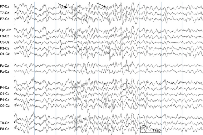
A related and dramatic version of the problem of the contaminated reference is seen in referential montages when the Cz electrode is chosen as the reference. In good electroencephalography laboratories, Cz is almost never chosen as the reference electrode for the referential montage. Very occasionally, however, Cz is the only available choice in a very active patient because there is no scalp muscle to generate muscle artifact under this midline electrode. Using a Cz reference can help avoid contamination with muscle artifact, but what happens when the patient falls asleep? Sleep vertex wave activity is maximally represented in the Cz electrode, and spindle activity is also plentiful there. For this reason, the sleeping patient in whom a Cz reference is used will manifest vertex waves and spindles in every channel (see Figure 5-26). Such a tracing can be difficult to interpret and is essentially unsatisfactory for most purposes.

Figure 5-26 A page of EEG sleep is displayed using a Cz reference. Because the Cz electrode is active with spindle and vertex-wave activity during sleep, this electrode position makes a poor choice for the reference electrode. Note that spindles and vertex waves appear to involve all channels on the page (arrows). Ironically, because of cancellation effects, the spindles are least well seen in the channels where their fields are strongest, C3 and C4.

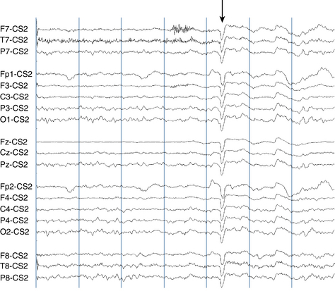
The second simple technique that can allow quick visual exclusion of a wave that arises from a contaminated reference is the phenomenon of a wave or signal that shows the exact same morphology in every channel. Higher voltage contamination will tend to have an identical appearance in all channels because that signal has been subtracted from each channel’s output. Figure 5-27 shows an example of such easily identifiable contamination.

Figure 5-27 An identical downward deflection is noted in all channels in the fifth second of the tracing (arrow). When a waveform of identical shape and amplitude is seen in a montage in which all channels are compared to a single reference, the simplest explanation is that the deflection arises from the reference.

The Laplacian Reference

The Laplacian reference is based on mathematical expressions that attempt to model the spherical surface of the scalp. This type of reference is occasionally used in routine EEG recordings but has a number of disadvantages. The Laplacian reference is a type of average reference in which the weight of each electrode in the average is affected by its distance from the electrode of interest. Electrodes that are closer to the electrode of interest are given more weight in the average, and more distant electrodes are given proportionally less weight. Because the more distant electrodes may only have a small impact on this type of weighted average and also because the mathematical expression for the full Laplacian reference is relatively cumbersome (and differs for each electrode on the scalp), some labs use a simplified version of the Laplacian reference. In this abbreviated version, only the immediately surrounding electrodes (a maximum of four) are used in the average; the more distant electrodes only make small contributions to the Laplacian because of their reduced weighting, and thus their values are discarded. Even this simplified technique has its weaknesses, such as the problem of how to handle electrodes that are on the edge of the electrode array such as O1 or Fp2 (typically only three electrodes are averaged in such instances). Likewise, noise in just one of the surrounding electrodes can have a fairly significant impact on this type of reference.

While use of the Laplacian reference can produce some satisfactory recordings, there is a fundamental disadvantage to this technique. As stated earlier, a basic tenet of careful interpretation of a referential montage is the importance of always knowing the exact reference in use. The problem with the Laplacian reference is that the question of “what is the reference?” is a constantly moving target because for every scalp electrode the reference is different. The fact that each electrode has a different reference may either slow down the analytic process of EEG interpretation or give the reader the incentive not to consider what the true reference is for every given channel, possibly leading to sloppy interpretation of complex electrical events. For these reasons, some feel that the Laplacian reference contributes little in the way of advantages over the average reference but presents a specific disadvantage to a reader who appropriately needs to know the composition of the reference for all channels at all times.

Using Colors in Montages

Digital computer systems offer laboratories the option of displaying different channels in different colors. For instance, some laboratories may choose to display all channels related to the left hemisphere in brown and all channels related to the right hemisphere in green. Although this may seem a like a good idea at first, this information should already be readily available based on channel position on the page. Because the eye is being trained to look for differences, the use of different colors may actually become a minor stumbling block given that the different colors create the appearance of a difference at the outset. To some, a darker color may look bolder during visual scanning, and therefore “bigger” than a lighter-colored channel, introducing an immediate bias toward one hemisphere. The author prefers montage setups in which a channel’s page position rather than its color is the indicator of brain position. Channel colors are most useful in the case of montages that alternate right- and left-sided channels. In general, when colors are used in montages, like colors are preferable for like brain regions.

The Appearance of Standard EEG Features in Different Montages

Each standard EEG feature has a characteristic appearance in the different EEG montages. The following figures review the appearance of eyeblink artifact, lateral eye movement artifact, the posterior rhythm, vertex waves of sleep, sleep spindles, and focal spikes in a variety of montages.

Figure 5-28 shows the typical appearance of eyeblink artifact in the AP bipolar montage. Because eyeblink artifact is caused by a large transient positivity in Fp1 and Fp2, the abrupt, downward-sloping waveforms seen in the four most anterior channels are characteristic for eyeblink artifact. The opposing phases seen in the anterior channels after the second eyeblink artifact are typical for lateral eye movements (see the figure caption for further explanation). In this figure, the posterior rhythm is seen in the posterior channels and even reaches as for forward as the F3-C3 and F4-C4 channels. Does this imply that the posterior rhythm is actually present in C3 and C4? The answer is no—the posterior rhythm is seen in F3-C3 because it disappears between F3 and C3. Because the two channels differ in that C3 picks up the posterior rhythm and F3 does not, the subtraction of the two channels still displays the posterior rhythm’s waveform.

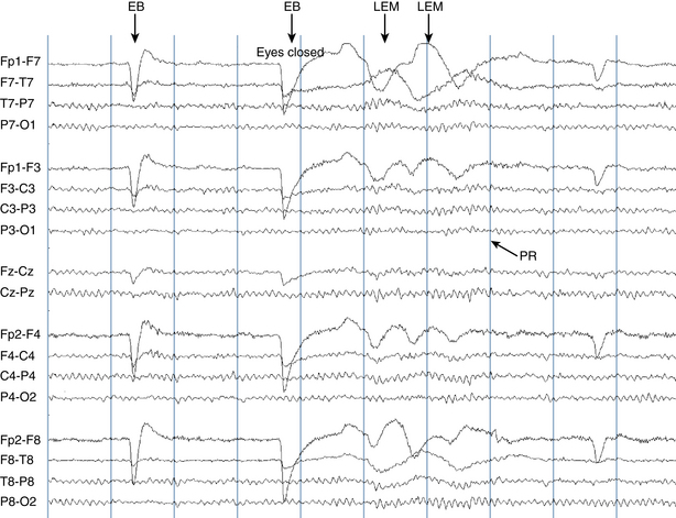
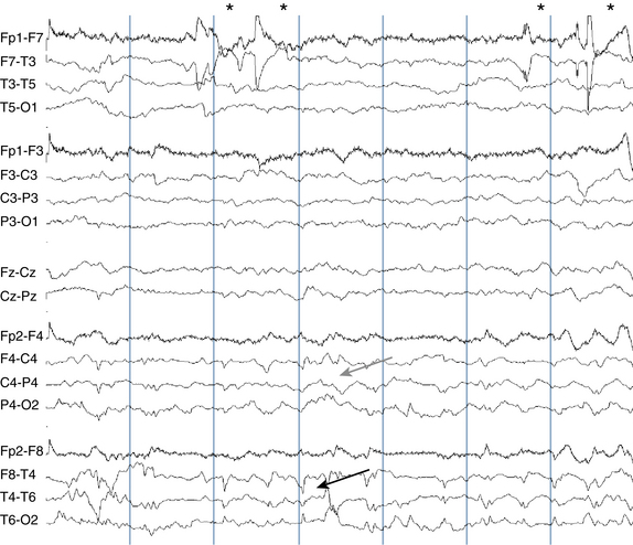
Figure 5-28 A page of wakefulness is shown in the anteroposterior (AP) bipolar montage. Eyeblink (EB) artifacts are the most prominent waveforms in this awake tracing, seen as a dramatic downward deflection most prominent in the top channel of each grouping of four channels in the AP bipolar montage. A smaller but similar deflection is also seen in the first channel of the midline electrodes (Fz-Cz). Eyeblink artifact is caused by an upward bobbing of the eyes that reflexively occurs during eye closure (Bell’s phenomenon). Because the anterior aspect of the eye is positively charged with respect to the posterior pole, eyeblinks result in a net positivity being detected by the frontal electrodes. Because the gradient (voltage difference) is typically greatest for eyeblink artifact between the most anterior electrodes (Fp1 and Fp2) and those directly posterior to them (F7, F3, F4, and F8), the eyeblink artifact waveform is almost always of highest amplitude in the most anterior channels (e.g., Fp1-F3 and Fp2-F4), as seen in this figure. Typically, this artifact is also visible, but to a lesser extent, in the next more posterior channels (e.g., F3-C3 and F4-C4). Because of the anterior source of the eyeblink potential, it is unusual to see a deflection posterior to these channels. Indeed, as is seen in this figure, the eyeblink deflection is not picked up in channels such as C3-P3 or T8-P8. At the end of the sixth second, high-voltage waveforms show opposing phases on the left compared with the right (lateral eye movement [LEM]). This type of artifact is caused by lateral eye movements and is discussed in more detail in Chapter 6. PR = posterior rhythm.

This same EEG page is shown in a variety of montages in Figures 5-29 through 5-35. It is worthwhile to take the time to identify each of the main elements of the awake EEG in each of these montages.

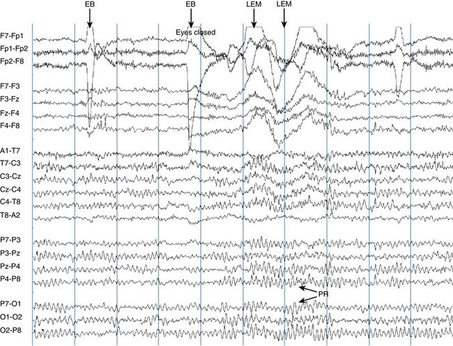
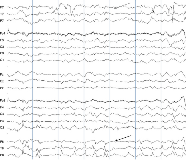
Figure 5-29 The same page of wakefulness as in Figure 5-28 is shown in the transverse bipolar montage. The eyeblink (EB) artifact is now essentially confined to the top three channels. Because the upward movement of the globes, which represents a net positive charge, is detected equally in Fp1 and Fp2, the amount of deflection in the Fp1-Fp2 channel is small. The Fp1 and Fp2 electrodes are, however, closer to the positivity of the eyeball as it bobs upward than the F7 and F8 electrodes. For this reason, the net positivity picked up by Fp1 being greater than at F7, the first channel, F7-Fp1, deflects upward. Likewise, because Fp2 detects more positivity than the F8 electrode, the third, Fp2-F8 channel, deflects downward. The posterior rhythm (PR) is well seen in the bottom three channels as expected, and also in the previous four channels, which link the left and right posterior temporal areas together, and even in the chain that links the left earlobe to the right earlobe (middle group of six channels). Only occasional fragments of the posterior rhythm are picked up in the chain that links the anterior temporal electrodes, F7 and F8 (the fourth through seventh channels nearer the top of the page). LEM = lateral eye movement.

Figure 5-30 A page of wakefulness is shown in the circumferential or “hatband” montage. The top 10 channels represent the circumferential portion of the display. The posterior rhythm (PR) is best seen in the middle channels of the circumferential portion, because these pass through the occipital regions. This montage is most easily scanned for symmetry through the midline visual axis formed by the O1-O2 channel. Eyeblink (EB) artifact is seen in the expected positions at the ends of the circumferential chain, because these represent the frontal region. LEM = lateral eye movement.

Figure 5-31 A page of wakefulness is shown in the anteroposterior referential montage using a CS2 reference (an electrode placed on the back of the neck). Recalling that in some patients electrocardiographic (EKG) artifact is present in the neck reference, rhythmic EKG artifact can be seen in all channels on this page. The fact that these “little spikes” appear with the same amplitude and morphology in every channel is a clue that they originate in the reference electrode rather than from the brain. In fact, on the basis of this artifact, the patient’s EKG rhythm can be counted out at 66 beats per minute. The field of the posterior rhythm is well defined, appearing, for the most part, in the posterior channels. Careful observation, however, shows that a small amount of the posterior rhythm (PR) is visible even in the most anterior channels. The astute reader will conclude that this is not because the posterior rhythm is actually present in the frontal areas but rather that the CS2 electrode is actually picking up the posterior rhythm to a small extent. This is not completely unexpected because the posterior rhythm’s field is maximum in the occipital regions, fairly close to the position of this neck electrode. The limitations of the use of the CS2 electrode evident in this page do not apply to all patients; in some patients, EKG artifact and posterior rhythm contamination are not seen in the CS2 electrode. EB = eyeblink; LEM = lateral eye movement.

Figure 5-32 The same page of wakefulness is shown in the AP referential montage using the chin as reference. Because in this patient, the chin does not pick up electrocardiographic (EKG) artifact, we do not see the EKG spikes as in the previous figure. Instead, in this patient, there is a small amount of muscle artifact in the chin, which causes this artifact to appear in every channel of this tracing. Note also that the posterior rhythm (PR) is appropriately completely absent from the Fp1 and Fp2 electrodes channels in this page (compare with the contamination phenomenon seen in the previous figure). EB = eyeblink; LEM = lateral eye movement; PR = posterior rhythm.

Figure 5-33 A page of wakefulness is shown in the anteroposterior referential montage using the nose as the reference. In this patient, the nose reference happens to be quiet, yielding an excellent quality tracing. Note the small spike-like artifact seen in the fourth second (under EB2 arrow). Because this small transient is similar in all channels, it can be identified as an artifact that originates in the nose reference. Again, eyeblink (EB) artifacts are seen confined to the anterior (Fp1, Fp2, F7, F3, F4, and F8) channels. The field of the posterior rhythm (PR) in this patient extends up to the C3 and C4 electrodes. Only occasionally are fragments of this rhythm seen as far forward as F3 and F4. As expected, the posterior rhythm cannot be identified in the frontopolar leads, Fp1 and Fp2. LEM = lateral eye movement.

Figure 5-34 A page of wakefulness is shown in the anteroposterior referential montage using the average reference. Some of the advantages and disadvantages of the average reference are evident in this page. The average reference yields a clean display from the point of view of being free of muscle artifact. However, note that the eyeblink (EB) artifacts seen in the anterior channels are being “answered” with upgoing waves in the posterior channels. This is an artifact of contamination of the average reference by the high-voltage eyeblink deflections. Likewise, the posterior rhythm (PR) can be seen in all channels, again an artifact of the effect of contamination of the average reference by the posterior rhythm (see further description of these problems in the paragraphs on the average reference). LEM = lateral eye movement.

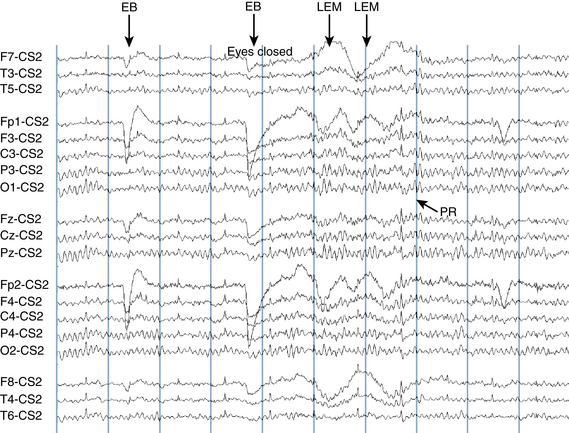
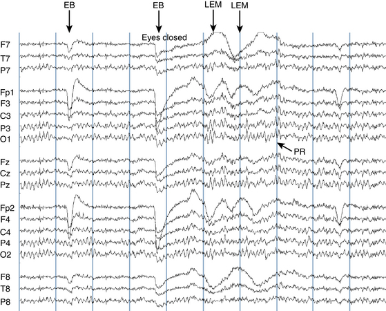
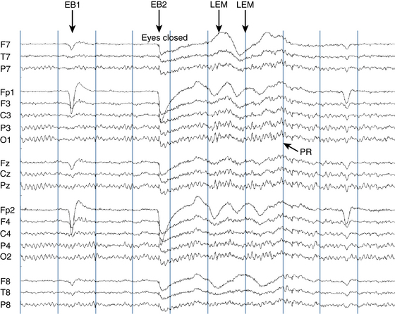
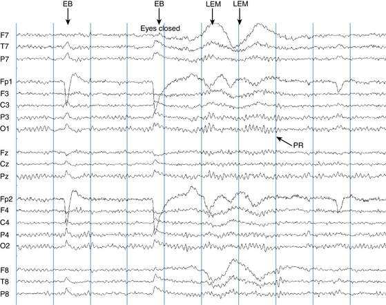
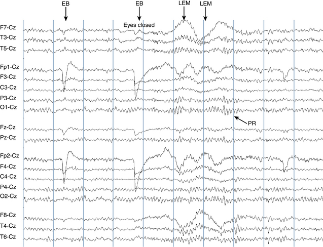
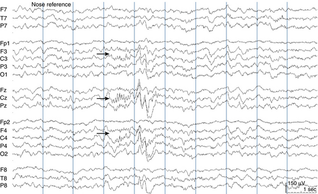
Figure 5-35 A page of wakefulness is shown in the anteroposterior referential montage using Cz as the reference. In this patient at this time in the tracing, the Cz electrode is relatively quiet. For this reason, this page appears to be of generally good quality, though note that the posterior rhythm can often be seen in all channels on the page, reflecting the fact that Cz is close enough to the back of the head that it intermittently picks up the posterior rhythm. This can be confirmed by looking at Figure 5-33 in which the posterior rhythm can often be discerned in the Cz-nose channel. Because all channels on this page are being compared to Cz, any activity that occurs in Cz has the potential to appear on every channel of the page. EB = eyeblink, LEM = lateral eye movement, PR = posterior rhythm.

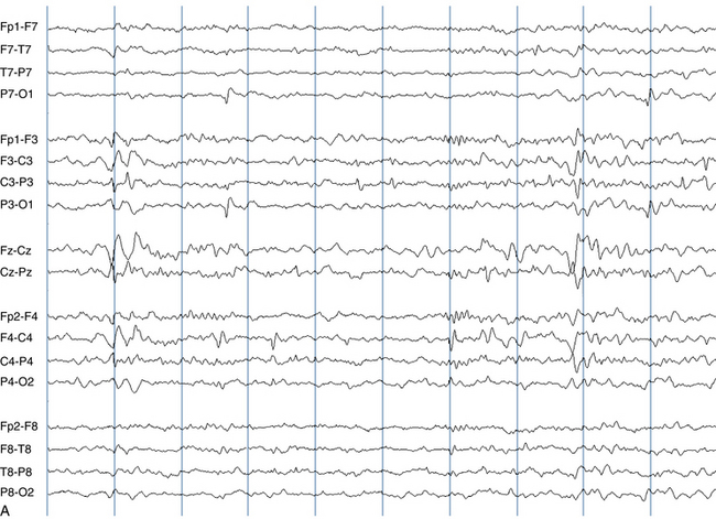
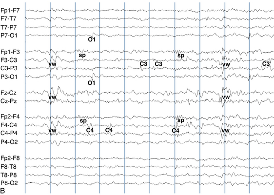
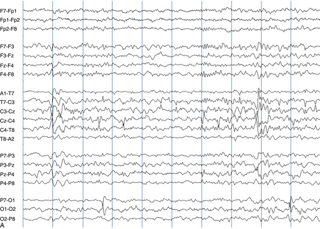
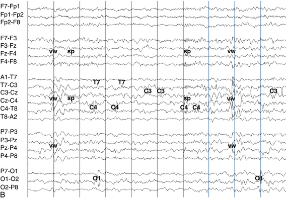
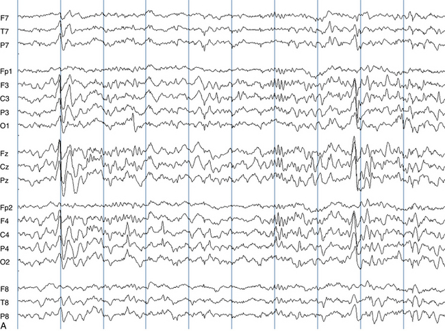
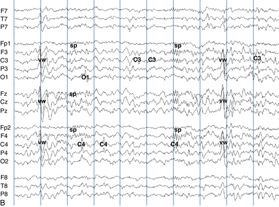
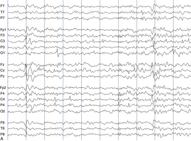
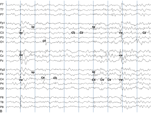
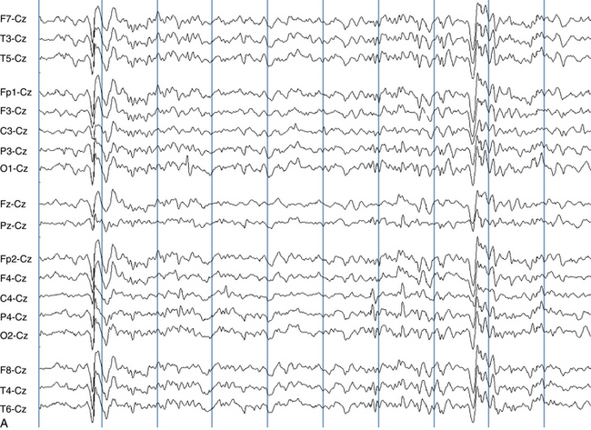
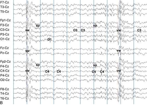
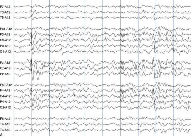
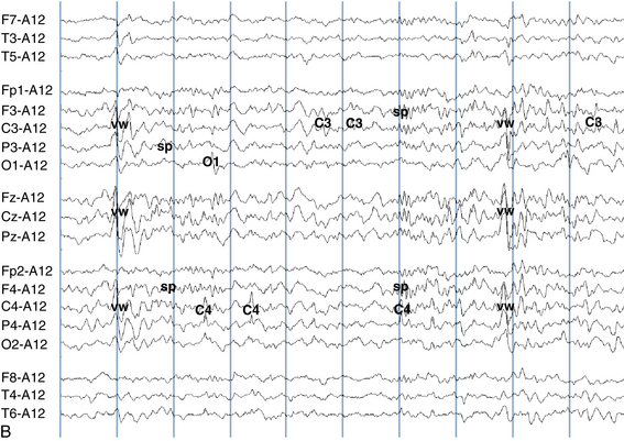
Figures 5-36 through 5-42 show the appearance of vertex waves, sleep spindles, and focal spikes from the same page of EEG recorded during sleep in the various montages (see figure captions for additional description). The top half of the figures show the EEG without markings to allow the reader to practice identifying key features. The bottom panel shows the same page with an “answer key” superimposed.

Figure 5-36 (A) This page of Stage II sleep displayed in an anteroposterior bipolar montage shows many features, including vertex waves of sleep, sleep spindles, a left occipital spike, and independent right and left central spikes. (B) The same page with labels: O1 = left occipital spike; sp = sleep spindle; vw = vertex wave of sleep; C4 = right central spike; C3 = left central spike.

Figure 5-37 (A) The same sleep segment is displayed in a transverse bipolar montage. Identify all of the various features in this transverse representation. Note that the vertex waves phase reverse in the Cz electrode suggesting that their voltage maximum is in the midline as expected, rather than off to one side. In contrast, the C3 and C4 spikes show clear phase reversals in those electrodes “off the midline,” clearly distinguishing them from the vertex waves. Likewise, the O1 spikes appear prominently at the bottom of the page. The spindles, which appear as low voltage 14-Hz waves, clearly involve both the frontal and central areas. (B) The same page with labels: O1 = left occipital spike; sp = sleep spindle; vw = vertex wave of sleep; C4 = right central spike; C3 = left central spike.

Figure 5-38 (A) The same page of sleep is displayed in a circumferential bipolar montage. The vertex waves and spindles are best seen on the bottom half of the page, which includes the parasagittal chains and the midline. The O1 spike appears prominently in the circumferential channels on the top half of the page. The C3 and C4 spikes are also evident. (B) The same page with labels: O1 = left occipital spike; sp = sleep spindle; vw = vertex wave of sleep; C4 = right central spike; C3 = left central spike.

Figure 5-39 (A) The same page of sleep is displayed using an anteroposterior referential montage using a nose reference. In this patient, the nose is electrically quiet during sleep and performs as an excellent reference electrode. The O1, C3, and C4 spikes are seen as upward deflections, although they do not “jump out” from the background as much as they do in bipolar montages. The fields of the vertex waves and spindles can easily be appreciated in this montage. (B) The same page with labels: O1 = left occipital spike; sp = sleep spindle; vw = vertex wave of sleep; C4 = right central spike; C3 = left central spike.

Figure 5-40 (A) The same page of sleep is displayed with an anteroposterior referential montage using the average reference. On this page the average reference gives a fairly good representation of EEG activity, but note that the spindle and vertex wave fields appear to be falsely broad because these waves have contaminated the average reference. In contrast, the O1, C3, and C4 spikes show up well against the background. (B) The same page with labels: O1 = left occipital spike; sp = sleep spindle; vw = vertex wave of sleep; C4 = right central spike; C3 = left central spike.

Figure 5-41 (A) Anteroposterior referential montage to the Cz electrode. Use of the Cz electrode as a reference is almost always a poor choice during sleep. Because sleep spindles, and especially vertex waves, appear strongly in the Cz electrode, this choice of reference spreads these waves across every channel, as is seen on this page. For example, the vertex waves appear in the temporal chains (top three and bottom three channels), although they are not really present in those locations. If one is able to ignore this effect, the location of some of the focal spikes can still be accurately discerned in this montage. (B) The same page with labels: O1 = left occipital spike; sp = sleep spindle; vw = vertex wave of sleep; C4 = right central spike; C3 = left central spike.

Figure 5-42 (A) This page shows a referential montage using a “mixture” or average of the earlobe electrodes, A1 and A2, as the reference. When the A1 and A2 electrodes are used as the reference electrodes, an alternative method used in some laboratories is to refer electrodes on the left side of the head to A1 and electrodes on the right side of the head to A2. (B) The same page with labels: O1 = left occipital spike; sp = sleep spindle; vw = vertex wave of sleep; C4 = right central spike; C3 = left central spike.