Chapter 9 Electrodiagnostic Medicine I
Fundamental Principles
Action Potential Generation
Nerve and muscle tissues are capable of generating an electrical difference across their cellular membranes, and can generate and sustain a propagating action potential. Interestingly, action potential generation is relatively similar between these two dramatically different tissues. The reader is strongly encouraged to read basic physiology texts25,28 to gain a more complete appreciation of the intricate relationship between excitable cells and their associated action potentials.
Resting Membrane Potential
All living cells generate an electrical potential across their membranes, with the intracellular region relatively negative compared with the extracellular region.28 This potential difference across the cell membrane is referred to as the resting membrane potential. The development and maintenance of the resting membrane potential can be explained by a simple model.
We can partition a beaker into right and left halves with an impermeable membrane containing multiple closed potassium channels. Assume this membrane separates two different concentrations of a potassium chloride (KCl) solution with a 10-mM concentration on one side and 100-mmol/L concentration on the other (Figure 9-1).17 Potassium chloride in solution exists as positive potassium (K+) ions (cations) and negative chloride (Cl–) ions (anions). A voltmeter (a device that detects potential differences) measuring the two solutions fails to detect a potential difference because there is a lack of physical continuity between the left and right halves of the beaker when the partition’s potassium channels are closed. In other words, the two solutions are electrically independent.
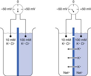
If we now open the membrane’s potassium channels, K+ cations will flow “down” their concentration gradient from the high (100 mm/L) to low (10 mm/L) ion concentration side of the beaker (see Figure 9-1). The potassium ions will continue this directional flow until there is a balance between (1) the forces of the physical concentration gradient difference driving potassium to the lower-concentration region, and (2) the electrical gradient opposing this directional ion flow. Because there are only potassium channels, the negative chloride ions cannot pass through the membrane and remain on their respective sides of the beaker. As more and more positive potassium ions leave one side of the beaker, there begins to develop an unbalanced or “excess” amount of negative charges (Cl–) on the high-concentration side of the beaker, with an equal buildup of “excess” positive charges (K+) on the other side of the beaker. The increasing net negative charge of the beaker half with the increasing number of unbalanced chloride ions begins to make it increasingly difficult for the positive potassium charges to leave the high-concentration side of the beaker. This is because the progressively building net negative charge increasingly attracts those remaining positive potassium ions. Similarly, a growing amount of positive potassium ions on the formerly low potassium concentration side of the beaker begin to increasingly repel additional potassium ions attempting to enter this side of the beaker.
The above simple example can be applied to all cells in the body, and in particular to nerve and muscle cells. A nerve’s axon will be used as a prototypical example, although the same principles apply to muscle cells. The nerve cell is known to have a specialized cell membrane permeable primarily to potassium and chloride ions in the resting state, because of proteinaceous transmembranous ion channels rendering the membrane selectively permeable (i.e., semipermeable).31 The potassium channels are referred to as passive, because they are always open and permit the free flow of this ion. Contained within the axon but incapable of crossing the cell membrane are large, negatively charged protein molecules. This negative charge attracts potassium ions from outside the cell to enter through the passive potassium channels, resulting in a buildup of potassium ions within the axon. This process continues until there is so much potassium within the axon that the continued entry of more potassium ions is prevented by the high intracellular potassium concentration, even though all the negative charges have not yet been electrically balanced. This is because the force of the accumulated potassium ions’ concentration gradient now attempting to drive potassium out of the cell is just large enough to balance the intracellular anions’ electrical force attracting potassium ions into the cell.
Nernst Equation
This formula can be rearranged to find the potential at which the electrical work just balances the concentration work (i.e., the dynamic equilibrium or resting membrane potential) by solving the above equation for Em

The above equation is more commonly known as the Nernst equation, and is a mathematical statement of the potential at which all the electrical and concentration forces are balanced in the cell’s resting state (i.e., the resting membrane potential).28,31 By substituting the actual values for the different variables and using the more familiar base 10 logarithm, the equation converts to the more recognizable form. Also, the approximate concentration ratio of intracellular to extracellular potassium is 20:1. The Nernst equation then becomes:
Sodium Pump
Experimentation has shown that the Nernst equation predicts the resting membrane potential quite well with different extracellular potassium concentrations, as long as the potassium concentration is relatively high. When the extracellular potassium concentration is low, there is a deviation of the resting membrane potential from that predicted, with a less-negative potential achieved. This finding suggests that another ion (sodium: Na+) has some influence on the resting membrane potential. It turns out that sodium has a very high extracellular concentration compared with intracellular ion concentration, which results in small quantities of sodium ions leaking into the membrane through a few passive sodium channels present in the cell’s membrane. This relative impermeability of positive sodium ions, combined with a high extracellular but low intracellular sodium ion concentration, and the resulting electrical drive to enter the cell (negative inside), would tend to “run down” the cell resting membrane potential over time. Fortunately, the cell has developed a mechanism whereby this run down is prevented. Located within the cell membrane is an energy-dependent sodium-potassium pump that pumps in potassium ions and pumps out sodium ions in just the right ratio to match the sodium ions entering and the compensatory potassium ions exiting the cell. Two sodium ions are extruded for every three potassium ions taken into the cell. The sodium-potassium pump maintains the exact ionic balance necessary to sustain a stable resting membrane potential by maintaining this 2:3 ratio.
Goldman-Hodgkin-Katz Equation
An important modification of the Nernst equation is the inclusion of ion permeability as being the primary influence on the cell’s transmembrane voltage. The greater an ion’s permeability, the more likely it is to influence the transmembrane potential. This is because the equilibrium potential of the most permeable ion in effect becomes the cell’s resting membrane potential. The equation accounting for the different permeability (designated as “p” in the equation below) factors is known as the Goldman-Hodgkin-Katz equation28,30,31:
Action Potential Generation
In addition to the passive (always open) potassium ion channels and relatively few passive sodium ion channels, there are also sodium and potassium ion channels within nerve and muscle cell membranes modulated by transmembrane voltage differences. These channels are voltage-gated because they open and close depending on the transmembrane voltage.25 Muscle and unmyelinated nerve contain both sodium and potassium voltage-gated channels. These voltage-gated sodium and potassium ion channels are closed at the resting membrane potential. If the transmembrane voltage changes toward a more depolarized direction (less negative) and reaches about 15 to 20 mV less negative than the resting membrane potential, the voltage-gated sodium channels open. This results in an increased permeability of the sodium ion, a process known as sodium activation. As noted above, the Goldman-Hodgkin-Katz equation predicts that the transmembrane potential shifts toward the sodium ion equilibrium potential. This massive shift in transmembrane potential is referred to as depolarization. After staying open for a short period, the sodium gates automatically close (sodium inactivation), with a return of the resting membrane potential again dictated by the resting state ion permeabilities (repolarization). In muscle and unmyelinated nerve membranes, a delayed opening of potassium voltage-gated channels occurs secondary to the depolarization and assists in repolarization.
Very few ions actually cross the membrane for sodium-induced depolarization or potassium-mediated repolarization. The region of membrane where there are large numbers of voltage-gated sodium channels in the open conformation acts as a so-called current sink for sodium ions to “sink,” or enter, the cell’s interior. This implies that a nearby source for the sodium ions must be present. The surrounding extracellular membrane region acts as the current source, thus permitting an ionic flow from the region surrounding the current sink. Sodium ions are thereby removed from the outside of the membrane surrounding the sink (making this region relatively more negative) and deposited on the inside of the cell (Figure 9-2). The newly introduced intracellular ions migrate to help neutralize some of the cell’s interior negative charges. This current flow, or charge transfer, from the extracellular to intracellular space is referred to as a local circuit current.17 The net effect of charge transfer is to make the cell’s interior less negative and exterior more negative, thereby shifting the transmembrane voltage in the more depolarized direction about the current sink. If the charge transfer is sufficient to depolarize the cell by approximately 15 to 20 mV, the membrane surrounding the sink is induced to permit sodium activation and hence undergo a significant depolarization. This process can then continue along the length of the cell.
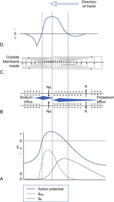
The above process creates an action potential spike at the original site of sodium activation. A mechanical, chemical, or electrical stimulus that causes the membrane potential to reach threshold over a localized region is all that is required to serve as the initiating stimulus of action potential generation. Once the process begins, it is self-sustaining as long as there are sufficient ion channels to repeat the depolarization process. The intracellular action potential is essentially a monophasic positive spike: –75 mV resting potential; +40 mV spike; return to resting –75 mV with sodium inactivation and potassium activation (see Figure 9-2). The membrane’s threshold value must be reached to generate the self-sustaining action potential that is the same at all regions of the membrane. This concept is referred to as the all-or-none phenomenon.
The nodes of Ranvier in myelinated nerves lack voltage-gated potassium channels and contain only voltage-gated sodium channels.47,48 The action potential actually “jumps” from one node to the next, creating an efficient means of action potential propagation that is referred to as saltatory conduction. Repolarization in myelinated nerve does not require a delayed potassium current. As noted above, the resting membrane potential is restored once the permeability of sodium is reduced. Passive “back-leak” sodium and potassium currents are thought to mediate the discharge of the membrane’s capacitance, which accumulates over time with multiple action potential discharges.
Physiologic Factors Affecting Action Potential Propagation
Gender
Only a few studies have attempted to investigate the difference in nerve conduction studies between men and women.3 Noted is a slight increase in the antidromic sensory nerve amplitudes for both the median and ulnar nerves recorded from the digits in women. Also, women demonstrate a greater nerve conduction velocity (NCV) for upper and lower limb nerves compared with men. Both of these differences, however, are eliminated when one considers limb length and digit circumference (see below).40
Aging
Several generalizations can be made regarding peripherally evoked sensory nerve action potentials (SNAPs) and aging. The conduction velocity demonstrates a consistent decline approximating 1 to 2 meters per second per decade.36 The duration of SNAPs is about 10% to 15% longer in persons aged 40 to 60 years, and 20% longer in those aged 70 to 88 years, compared with persons aged 18 to 25 years.8 Compared with the 18- to 25-year-old group, the SNAP amplitude is one half and one third, respectively, for the 40- to 60-year-old and 70- to 88-year-old groups. The distal sensory latencies reveal a similar prolongation with age. There is a suggestion that the median and radial nerves do not demonstrate considerable alteration with age.19 At present, there is disagreement as to the magnitude of change in SNAP parameters induced by the aging process.
The results of aging on conduction velocity have been examined in a number of upper and lower limb nerves. Motor NCVs reveal similar changes to those described for sensory nerves. The newborn’s motor NCVs are about half of adult values, which are reached by 3 to 5 years of age.2 After the age of 50 years, the conduction velocity of the fastest motor fibers progressively declines by approximately 1 to 2 m/s per decade. There is a concurrent increase in the distal motor latency and decrease in the motor response’s amplitude with advancing age. H-reflex latency demonstrates little alteration with aging in the healthy elderly.20 The decrease in amplitude is difficult to ascertain clinically because of the wide range of normal H-reflex amplitudes and the central effects on amplitude that are difficult to control and quantify.
Digit Circumference
Females consistently demonstrate significantly higher antidromic SNAP amplitudes for the median and ulnar nerves recorded from the second and fifth digits.3 A negative linear correlation exists between finger circumference and amplitude for these two nerves. It is known that as the distance between the recording electrode and neural generator increases, the amplitude precipitously declines. Increasing the circumference of the finger displaces the electrode further from the nerve. Because men have significantly larger finger circumferences than women, this appears to explain the difference in SNAP amplitudes. There is no evidence that this difference is due to an intrinsic neural difference between male and female nerves.
Height
Several investigations have documented slower lower limb NCVs in taller compared with shorter individuals.9,33 This difference is independent of the limb’s temperature or subject’s age. The etiology of this finding is unknown. Distal nerve tapering or an abrupt change in axon diameter has been speculated to account for this finding, but the exact etiology has not been definitively identified.14,46
Temperature
Temperature is one of the most important factors influencing nerve conduction studies. As the temperature of the nerve is lowered, the amount of current required to generate an action potential increases. This decreased excitability is a direct temperature effect on the nerve’s action potential–generating mechanism at the nodes of Ranvier, and not a result of membrane resistance changes. The transmembrane resistance is not increased by a drop in temperature.26,27 In addition to excitability, the configuration of an action potential is profoundly affected by a drop in temperature.
The action potential’s amplitude, rise time, and fall time all increase as the nerve’s temperature declines. The time required for the action potential of a cold nerve to reach its peak depolarization from the resting membrane level increases approximately 33%.38 Similarly, the time necessary for the action potential to return to its resting level is also increased, but much more so than the rise time (69%). Because both the SNAP duration and the spike height increase, the area of the SNAP increases dramatically at lower temperatures.
The first detailed investigation of temperature effects on NCV in human nerves revealed an NCV to temperature correlation of 2.4 m/s per °C for median and ulnar motor conduction.24 With every 1° C drop in temperature, there was a 2.4 m/s decrease in the conduction velocity. Reductions in conduction velocity for upper limb motor nerve fibers have also been found to approximate a decrease of 4% or 5% per °C.10,29 Correction factors using subcutaneous and intramuscular readings are equally correct, but it is more convenient and less painful to use surface measurements.22
In the upper limb, the relationship between temperature and NCV has been investigated for the surface temperature range of 26° C to 33° C, measured at the midline of the distal wrist crease. Calculations reveal that for median motor and sensory nerves, NCV is altered 1.5 and 1.4 m/s per °C, respectively, while the distal latency for both nerves changes about 0.2 ms/°C.21–23 The ulnar nerve demonstrated motor and sensory temperature relationships of 2.1 and 1.6 m/s per °C, respectively, and a distal motor and sensory latency correlation of 0.2 ms/°C.
Waveform Configuration Generation
The current flow created by a depolarized region of membrane (current sink) is associated with a specific pattern of voltages known as isopotential lines (Figures 9-2 and 9-3).13 Recording a voltage at any point in space along an isopotential line results in the same voltage being recorded. As one moves further from the current sink, the corresponding voltage and the current density also decrease. The pattern of isopotential lines in space creates three distinct voltage regions. The current sink is associated with a negative voltage, while the two surrounding (leading and trailing) current sources are considered zones of relative positive voltage. Separating the current sink zone from the current sources are zero isopotential lines. These lines correspond to regions of zero voltage associated with that portion of the recorded waveform crossing the baseline (see Figure 9-3).
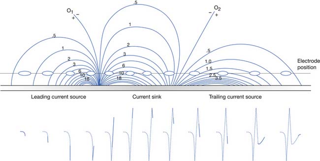
An action potential with its local circuit current and associated isopotential lines propagating past an electrode can be considered essentially equivalent to a stationary action potential sequentially sampled by a recording electrode passing through its electrical field (see Figure 9-3). The latter situation is used as an example for discussion purposes because it is easier to visualize the ensuing action potential waveform.
Suppose a propagating nerve or muscle action potential is frozen for an instant in time. A characteristic pattern of isopotential voltage lines is described in the region surrounding the nerve or muscle. A recording electrode can then be moved through the activated tissue’s electrical field to simulate a propagating action potential (see Figure 9-3). The final waveform configuration associated with an action potential propagating along a straight portion of nerve or muscle is a triphasic waveform with a large negative spike flanked by an initial large and subsequent small terminal positive phase. For discussion purposes, positive is denoted by a downward cathode ray tube (CRT) deflection, while an upward CRT deflection designates a net negative potential difference between the two recording electrodes. This example implies that for both nerve and muscle, when an action potential approaches, reaches, and then travels past a recording electrode, the fundamental waveform configuration is triphasic. These same simple principles can be applied to understand the generation of all waveforms observed during the electrodiagnostic medicine examination.
Nerve and Muscle Waveform Configurations and Characteristics
Nerve Potentials
Sensory Nerve Action Potentials
Clinical Recordings
SNAPs can be obtained with either antidromic or orthodromic techniques.8 The term antidromic implies that the induced neural impulse propagates along the nerve in a direction opposite to its physiologic direction; for example, stimulating the median nerve at the wrist and recording the ensuing response from the second or third digit. A nerve will conduct an impulse proximally and distally from the point of stimulation by a depolarizing current. On the other hand, stimulating the median sensory fibers on the second digit and recording from the wrist is an example of an orthodromic technique. In orthodromic recordings, the sensory fiber impulses are detected at a site proximal to the stimulus as they travel physiologically from a distal to a more proximal region. Antidromically obtained SNAPs are usually larger and hence easier to assess, because the recording electrodes are in close proximity to the proper digital nerves than when a recording electrode is placed over the median nerve at the wrist for orthodromic techniques. Mixed nerve responses can have a component of both orthodromic and antidromic waveforms. For example, midpalm stimulations recorded at the wrist are a combination of orthodromic sensory and antidromic motor responses.
SNAP Configuration
Antidromic and orthodromic bipolar SNAP waveform recordings are typically biphasic rather than triphasic. The biphasic, negative-positive potential is a result of the bipolar recording technique and not a violation of volume conductor theory. Biphasic SNAP waveforms can best be understood by use of bipolar and referential recording montages for median nerve stimulation at the wrist (Figure 9-4).13 The median SNAP is indeed a triphasic waveform and conforms to the principles of volume conduction, but only appears biphasic because of the recording montage used.
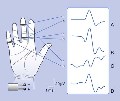
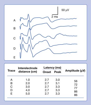
It is also possible to predict the optimal interelectrode separation to maximize the biphasic potential’s amplitude in the bipolar recording.17 The critical factor in this instance is the rise time, baseline to negative peak, of the biphasic potential, because it is this parameter that defines the waveform’s maximum amplitude. The recording electrodes must be located at a distance greater than the action potentials’ spatial extent, represented by the rise time duration. The rise time of most SNAPs approaches 0.8 ms, which represents a longitudinal extent of 40 mm for an action potential conducting at 50 m/s (50,000 mm/1000 ms = D/0.8 ms; D = 40 mm). If the two recording electrodes are separated by a distance less than 40 mm, some similar information regarding the main peaks of the waveforms recorded by both recording electrodes (active and reference) results in mutual cancellation of data, producing a potential with a smaller amplitude. A portion of the nerve will be depolarizing under the reference electrode while still in some degree of depolarization under the active electrode. At interelectrode separations greater then 40 mm, the biphasic potential’s negative peak amplitude will no longer grow, but the terminal positive phase will enlarge slightly and might change its configuration. These findings can be demonstrated by varying the distance between recording electrodes and observing the ensuing results (Figure 9-5). In effect, as the recording distance decreases below 40 mm, the amplitude of the recorded waveform declines and the peak latency shortens.
Muscle Potentials
Needle Insertional Activity
Normal Insertional Activity
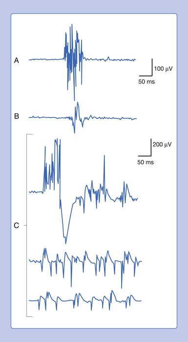
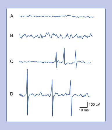
Placing a needle (monopolar or standard concentric) recording electrode into healthy muscle tissue and advancing it in quick but short intervals results in brief bursts of electrical potentials referred to as insertional activity (Figure 9-6, A).14 The observed electrical activity is believed to result from the needle electrode mechanically depolarizing the muscle fibers surrounding its leading edge as it pierces and deforms the tissue. Minimal and localized muscle tissue damage may occur from direct needle trauma and is the basis for the synonymous term of injury potentials. The purpose of including insertional activity analysis as part of the electromyographic examination is that the probing needle might provoke transient and/or sustained abnormal potentials associated with membrane instability before this abnormal activity with the muscle at rest.
Decreased Insertional Activity
Muscle that has been replaced by fibrous tissue, or that is otherwise electrically inexcitable, can no longer generate electrical activity. Consequently, the needle electrode is incapable of mechanically depolarizing this tissue. The result is that few, if any, electrical waveforms will be detected after needle movement (Figure 9-6, B).
Increased Insertional Activity
Practitioners have noted that insertional activity can appear to persist after needle movement cessation. This finding has led to the term increased insertional activity. In disease states where the muscle is no longer connected to its nerve or the muscle membrane is inherently unstable from primary muscle pathology or abnormal ion channels, the increased insertional activity completes a temporal continuum from the previously normal insertional activity to the development of sustained membrane instability (Figure 9-6, C). Practitioners differ as to the significant differences if any between increased insertional activity and positive sharp waves.
End-Plate Potentials
Miniature End-Plate Potentials
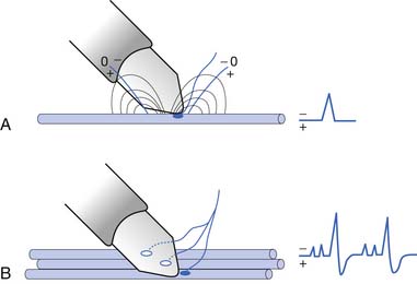
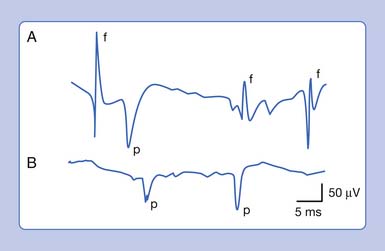
An active needle electrode located in the end-plate region can record two distinct waveforms. One of the waveforms is a short-duration (0.5 to 2 ms), small (10 to 50 μV), irregularly occurring (once every 5 seconds per axon terminal), monophasic negative waveform.14 These potentials represent the random release of acetylcholine vesicles. Volume conduction theory would suggest that for a potential to be monophasic and negative, the current sink would have to start and finish within the active electrode’s recording region (Figure 9-7, A).Clinically, multiple miniature end-plate potentials (MEPPs) are usually observed with an intramuscular recording electrode, and the sound is referred to as end-plate noise resembling a “seashell murmur” (Figure 9-7, B).
End-Plate Spikes
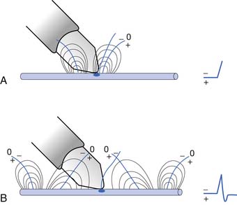
A second waveform that can be detected with an active needle electrode placed in the end-plate region is relatively short in duration (3 to 4 ms), of moderate amplitude (100 to 200 μV), irregularly firing, and biphasic with an initial negative deflection.14 The biphasic potential has an initial negative phase, produced when a current sink originates in the vicinity of the active electrode and then propagates away (Figure 9-8). Triphasic end-plate spikes might also occur if the active electrode induces an action potential in the terminal axon but the electrode’s recording surface is some distance from the end plate. End-plate spikes and MEPPs are frequently observed together, as they arise from the same region (Figure 9-9).
Single Muscle Fiber
The single muscle fiber generates three waveforms that are at times difficult to separate: end-plate spikes, positive sharp waves (PSW), and fibrillation potentials. End-plate spikes can have the identical morphology of PSW and fibrillation potentials. The major key to separating them is that PSW and fibrillation potentials have a regular firing rate and can slowly trail off. End-plate spikes usually are irregular. The single muscle fiber’s extracellular waveform configuration, like nerve tissue, depends on the characteristics of the muscle’s intracellular action potential. A muscle’s action potential is approximately 4 to 20 times longer than a nerve’s, because of the prolonged repolarization process.14 Aside from the longer duration of local circuit currents compared with neural tissue, the concept of a current sink surrounded by two source currents (source-sink-source) remains unchanged. A triphasic waveform with a small terminal phase should then be recorded from an extracellular active electrode placed adjacent to a propagating single muscle fiber action potential at some distance from the end-plate region (Figure 9-10).
Motor Unit Action Potential Configuration
Amplitude and Rise Time
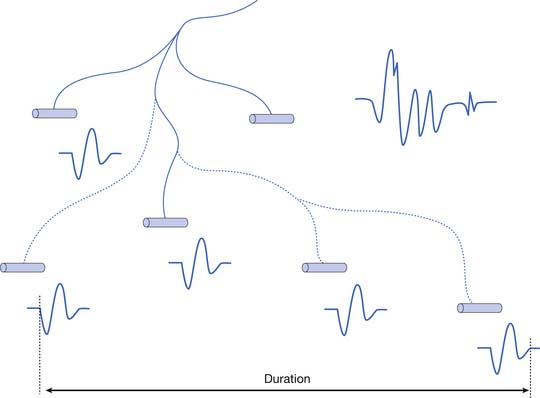
The MUAP configuration can be described in terms of its amplitude (maximum peak-to-peak CRT trace displacement), rise time (temporal aspect of a potential’s peak), duration (departure from and return to baseline), and number of phases (baseline crossings plus one) (Figure 9-11). The amplitude of potentials declines exponentially with increases in distance from the current generator. This occurs because the surrounding muscle and its supportive tissues act as a high-frequency filter to impede potentials that change rapidly over a short period. As a result, the peak-to-peak MUAP amplitude is believed to arise from fewer than 12, and possibly just 1 or 2, single muscle fibers located within 0.5 mm of the electrode’s recording surface. Small movements in the needle electrode frequently change the amplitude dramatically as the needle gets closer or farther away from the motor units.
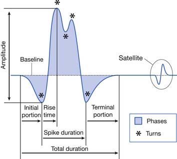
Duration
The MUAP duration depends on the shortest and longest lengths of terminal axons from the point they separate from the parent nerve to the end plate. The duration of the MUAP also depends on the conduction velocities of the terminal axons and individual muscle fibers with respect to the recording electrode, and the muscle fiber length (see Figure 9-11).6,7 The duration of an MUAP is the most sensitive clinical parameter that can be routinely quantified to diagnosing disease. Small movements in needle electrode position have a negligible effect on the duration of the MUAP, which is in contrast to the amplitude and rise time.
Phases
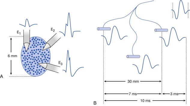
As previously stated, the single muscle fiber action potential usually has a triphasic appearance when recorded outside the end-plate zone and away from the tendinous insertion. The voltages from all the single muscle fibers belonging to one motor unit summate to yield an MUAP that is also usually triphasic: positive-negative-positive. This voltage summation does not always produce a smooth result, and small serrations, or turns, can occasionally be seen as part of the major phase of an MUAP (see Figure 9-11). The number of phases is defined as the number of CRT trace baseline crossings plus one. Normal MUAPs are considered to have four or fewer phases. MUAPs with five or more phases are called polyphasic potentials. Recordings of multiple MUAPs from normal muscle tissue can have between 12% (concentric needle) and 35% (monopolar needle) polyphasic potentials, depending on the type of recording electrode used.14 Slightly different MUAP configurations can be expected, depending on the exact location of the recording electrode with respect to different single muscle fibers within the motor unit territory (Figure 9-12). Satellite potentials are late waves that are linked to the rest of the waveform.
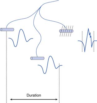
Pathology can also alter the number of phases an MUAP waveform can have. The motor unit can be affected in two general ways after injury or disease: a pathologic condition may affect either the anterior horn cell or peripheral nerve (including the neuromuscular junction), or the muscle fibers comprising the motor unit. If the neural component of a motor unit is compromised severely enough to experience degeneration, all the muscle fibers innervated by the parent nerve will become denervated. These denervated muscle fibers induce nearby terminal axons of intact nerves to send out neural projections to reinnervate the orphaned muscle fibers most likely through neurotrophic factors. Through collateral sprouting, the total number of muscle fibers belonging to a specific motor unit may increase dramatically (Figure 9-13). Neurogenic diseases can lead over a period to larger-amplitude, longer-duration, and highly polyphasic MUAPs.
If the muscle fibers comprising a motor unit undergo random degeneration, such as occurs in some myopathies, there is a decrease in the total number of fibers belonging to that motor unit (Figure 9-14). A decrease in muscle fiber numbers would result in a reduction of the overall MUAP amplitude, including its initial baseline departure and subsequent return. If the initial baseline departure of the original MUAP and its subsequent return to baseline decline in magnitude, this portion of the waveform can no longer be observed (assuming the amplifier’s gain is not increased). As a result, the total duration of the MUAP would correspondingly appear to decrease. Finally, the dropout of single muscle fiber waveforms would produce less voltage with respect to the spatial summation of single fiber potentials. Fewer muscle fibers could lead to “gaps” in the MUAP waveform, causing an increase in the number of phases. Consequently, a primary myopathic process tends to yield shorter-duration, highly polyphasic, low-amplitude MUAPs.
Compound Muscle Action Potential
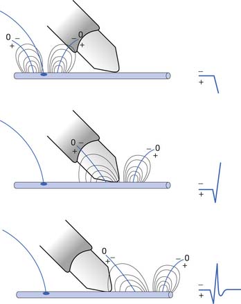
To elicit a CMAP from a particular muscle, the active electrode is located on the skin’s surface directly over the muscle’s end-plate region, or “motor point.”14 The end-plate region typically lies midway between the muscle’s origin and insertion. The reference electrode is usually placed on or distal to the tendinous insertion of the muscle, so as not to record electrical activity from the activated muscle. Stimulating the peripheral nerve innervating the muscle under investigation will result in a relatively large, biphasic waveform with an initial negative deflection (Figure 9-15).
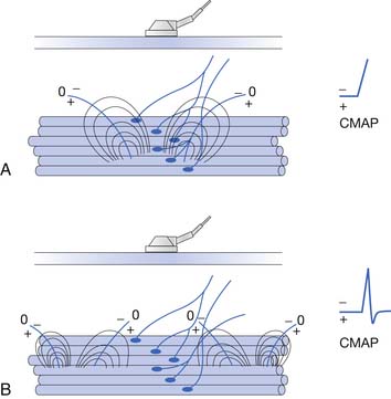
Occasionally, a positive deflection can precede the negative phase of the CMAP. Volume conductor theory can explain this observation (Figure 9-16). The active electrode may not be located directly over the motor point but displaced longitudinally away from it. An active electrode located off the motor point will first record some portion of one of the source currents “feeding” the current sink. Recall that the leading portion of the source current will result in a positive deflection of the CRT trace. As propagation ensues in the muscle, the current sink will eventually reach the active electrode, resulting in a negative deflection. Finally, the terminal source current is detected, producing a positive deflection. Instead of the anticipated biphasic potential, a triphasic positive-negative-positive waveform is recorded. Relocating the active electrode over the anticipated motor point region will usually remedy the situation.
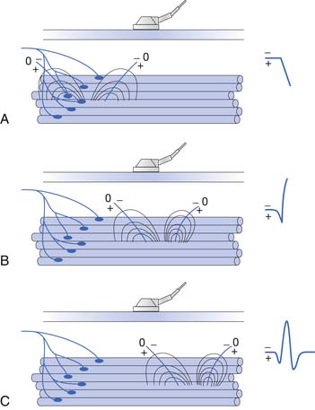
FIGURE 9-16 A, Relocating the active electrode in Figure 9-15 off the motor point results in a compound muscle action potential with an initial positive deflection, as some of the muscle’s action potentials no longer originate under the electrode but propagate toward it. B, When the main negative sink reaches the electrode, the potential’s main negative spike is detected. C, Finally, the terminal positive source currents are recorded, generating the potential’s terminal positive phase.
(Redrawn from Dumitru D, Amato AA, Zwarts MJ: Electrodiagnostic medicine, ed 2, Philadelphia, 2002, Hanley & Belfus, with permission.)
This situation is complicated by the interaction of near-field and far-field waveforms. At times, a far-field waveform might predominate, depending on the active and reference electrodes’ respective locations. This can lead to a waveform with an initial positive deflection or a varying negative waveform onset (so-called false motor points). The interested reader is encouraged to explore these fascinating concepts of near-field and far-field waveform interactions.14
Muscle Generators of Abnormal Spontaneous Potentials
Fibrillation Potentials
In vitro observations have shown that approximately 6 days after denervation, a skeletal muscle fiber’s resting membrane potential decreases to a less negative level of −60 mV compared with the normal value of –80 mV.5,45 Additionally, the resting membrane potential begins to oscillate. Because the threshold level for initiating the all-or-none action potential is now closer to the new resting membrane potential, an oscillating membrane potential will eventually reach the threshold level. Once threshold is achieved, a propagating action potential is induced, referred to as a fibrillation potential. The repolarization phase of denervated muscle results in a temporarily more hyperpolarized (–75 mV or more) level than the newly established resting membrane potential of –60 mV. When the hyperpolarized membrane level (–75 mV or more) returns to its resting membrane level of –60 mV, an action potential is again produced. This process regularly repeats, resulting in the commonly observed spontaneous and regularly repetitive discharge of fibrillation potentials. Irregularly firing fibrillation potentials occur at times, and are less well understood but thought to arise from spontaneous depolarizations within the transverse tubule system.
Fibrillation potentials are simply spontaneous depolarizations of a single muscle fiber, and demonstrate waveform configurations similar to those of single muscle fibers that are voluntarily activated (Figure 9-17). Fibrillation potentials are typically short in duration (less than 5 ms), less than 1 mV in amplitude, and fire at rates between 1 and 15 Hz. They have a typical sound, likened to a high-pitched tick like “rain on a tin roof,” when amplified through a loudspeaker. When the recording electrode is located in the previous end-plate zone of a denervated muscle, fibrillation potentials can be biphasic with an initial negative deflection. A recording electrode outside the end-plate zone, but far from the tendinous region, will detect fibrillation potentials that are triphasic (positive-negative-positive).
It is possible to generate waveforms with similar configurations to fibrillation potentials while examining healthy muscle tissue. Specifically, inadvertently irritating the terminal axon or end-plate zone with the electrode’s shaft, and evoking end-plate potentials while simultaneously recording at some distance from the end-plate zone, will generate triphasic end-plate spikes that are identical in appearance to fibrillation potentials (Figure 9-18).14 This is understandable because both waveforms are single muscle fiber discharges. The key to identification is the rapid and irregular discharge of end-plate spikes, while fibrillation potentials fire much slower and very regularly.
Positive Sharp Waves
PSWs are waveforms that can be recorded from a single muscle fiber having an unstable resting membrane potential secondary to denervation or intrinsic muscle disease. Typically, they have a large primary sharp positive deflection followed by a small negative potential. These potentials are called PSWs (see Figure 9-17). This waveform is thought to have the same clinical significance as a fibrillation potential, in that it is a single muscle fiber discharge. Amplified through a loudspeaker, PSWs have a regular firing rate (1 to 15 Hz) and a dull thud sound. Their durations range from several milliseconds to 100 ms or longer. Although commonly observed to fire spontaneously, PSWs can be provoked by electrode movement, as can fibrillation potentials.
A number of other waveforms can be observed that have the configurations resembling a PSW. An MUAP recorded from the tendinous region can also have an initial positive deflection followed by a negative potential, because the current sink cannot pass beyond the recording electrode.14 It is also possible for the recording electrode to damage a number of muscle fibers in close proximity to the recording surface, again preventing an action potential from passing its recording surface, resulting in a primarily positive potential. These two potentials can be distinguished from a PSW in that they are MUAPs and subject to voluntary control, whereas a PSW is not. Asking the individual to contract and relax the muscle under investigation should demonstrate that the waveform has a variable firing rate. A PSW typically fires at a regular rate and is not under voluntary control. If any doubt remains, the electrode should be repositioned until successful recordings are obtained. PSWs and fibrillations will usually disappear when the needle electrode is moved a small distance such as 1 to 5 mm, while a motor unit will usually remain on the screen and change shape. This is because the fibrillation potential is generated by a very small electrical charge from only one muscle fiber, whereas an MUAP is generated by hundreds of muscle fibers covering an area of 1 to 3 cm2.
Transient runs of “PSW-appearing potentials” can be seen in healthy skeletal muscle, particularly in the paraspinal and hand or foot intrinsic muscles. The “nonpathologic” PSWs are thought to arise because the needle electrode is oriented in such a manner as to irritate an end plate’s terminal axon, but extend along the muscle fiber while compressing the tissue and preventing action potential conduction.14 The induced end-plate spike appears like a PSW, but it displays a relatively rapid and irregularly firing rate characteristic of end-plate spikes (see Figure 9-18). Sustained PSWs are more significant than unsustained PSWs.
There is debate as to whether fibrillation potentials are distinct from PSWs, and if so, whether this has any clinical significance. Fibrillations potentials have been characterized as the spike form or biphasic waveform.12 There is strong evidence that the PSW is a fibrillation that has a different shape primarily because the needle electrode is touching the fibrillating muscle cell, altering the muscle membrane and consequently the shape of the waveform.15,16 It is unlikely that there is any clinically significant difference between the two.
Complex Repetitive Discharge
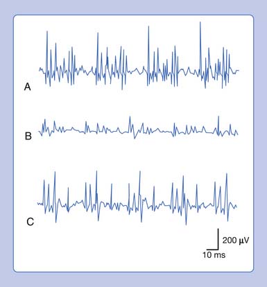
A complex repetitive discharge (CRD) is a spontaneously firing group of action potentials (formerly called bizarre high-frequency discharges or pseudomyotonic discharges) and requires a needle recording electrode for detection.14 The configuration of these waveforms is that they are continuous runs of simple or complex spike patterns (fibrillation potentials or PSWs) that regularly repeat at 0.3 to 150 Hz. The repetitive pattern of spike potentials has the same appearance with each firing, and bears the same relationship with its neighboring spikes (Figure 9-19). A distinct sound, likened to that of heavy machinery or an idling motorcycle, is produced by the firing of CRDs. In addition to the sound and repetitive pattern, a hallmark of these waveforms is that they start and stop abruptly. CRDs might begin spontaneously or be induced by needle movement, muscle percussion, or muscle contraction. Nerve block and curare do not abolish CRDs, suggesting that the origin of these potentials is within the muscle tissue. Single-fiber and standard electromyographic studies suggest CRDs are generated by an ephaptic activation of adjacent muscle cells.12 Detection of these waveforms usually suggests that a chronic process has resulted in a group of muscle fibers becoming separated from their neuromuscular junctions. They may be associated with a currently active disease or be the residua of a past disorder.
Myotonic Discharges
The phenomenon of delayed muscle relaxation after muscle contraction is referred to as myotonia or action myotonia.14 The finding of delayed muscle relaxation after reflex activation, or induced by striking the muscle belly with a reflex hammer, is called percussion myotonia. Clinical myotonia is usually accentuated by energetic muscle activity after a rest period. Continued muscle contraction lessens the myotonia and is known as the “warmup.” It is thought that cooling the muscle accentuates myotonia, but this finding has only been objectively documented in paramyotonia congenita.
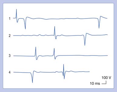
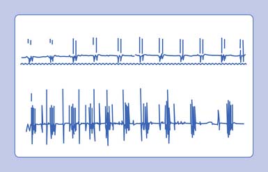
Myotonic discharges can present in one of two waveform types (Figure 9-20). The myotonic potential induced by needle electrode insertion usually assumes a morphology similar to that of a PSW or a fibrillation potential. It is thought that the needle movement induces a repetitive firing of the unstable membranes of multiple single muscle fibers. This is because the recording needle is thought to have damaged that portion of the muscle fiber with which it is in contact. Regardless of the waveform type, the hallmark of myotonia is the waxing and waning in both frequency and amplitude. The myotonic discharge has a characteristic sound, likened to that of a dive bomber and easily recognized. Amplitudes range from 10 to 1 mV, and firing rates from 20 to 100 Hz.42
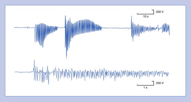
FIGURE 9-20 A run of myotonic potentials demonstrating the waxing and waning nature of the discharge.
Myotonic discharges can occur with or without clinical myotonia. The observation of these potentials requires needle movement or muscle contraction. These waveforms persist after nerve block, neuromuscular block, or frank denervation. This suggests that their site of origin is the muscle membrane itself, and they appear to be due to a channelopathy. Although the exact mechanism of myotonic discharge production remains unclear, it is proposed that decreased chloride conductance is responsible at least in part for the findings in myotonia congenita.14 Myotonic discharges are not specific for any one disorder. In addition to the myotonic disorders of muscle, myotonic discharges can also be detected occasionally in acid maltase deficiency, polymyositis, drug-induced myopathies, severe axonal neuropathies, and at times in any nerve or muscle disorder.
Neural Generators of Abnormal Spontaneous Potentials
Fasciculation Potentials
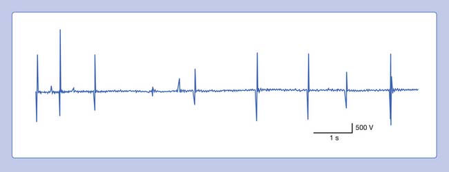
The visible spontaneous contraction of a portion of muscle is referred to as a fasciculation. When these contractions are observed with an intramuscular needle recording electrode, they are called fasciculation potentials.4,14 A fasciculation potential is the electrically summated voltage of depolarizing muscle fibers belonging to all or part of one motor unit. Occasionally, fasciculation potentials can be documented only with needle electromyography, because they lie too deep in muscle to be seen.
Fasciculation waveforms can be characterized with respect to phasicity, amplitude, and duration (Figure 9-21). Their discharge rate (1 Hz to many per minute) is irregular and occur randomly. They are not under voluntary control, nor are they influenced by mild contraction of the agonist or antagonist muscles. The site of origin of fasciculation potentials remains unclear, although it appears that there are three possible sites: the spontaneous discharge might arise from the anterior horn cell, or along the entire peripheral nerve (particularly the terminal portion), or at times within the muscle itself.
Myokymic Discharge
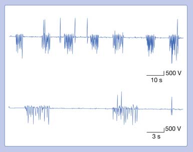
Myokymia is frequently readily observable as vermicular (bag of live worms) or rippling movement of the skin. It is usually associated with myokymic discharges.14 The myokymic discharge consists of bursts of normal-appearing motor units with interburst intervals of electrical silence. Typically, the firing rate is 0.1 to 10 Hz in a semirhythmic pattern. Two to 10 potentials within a single burst can fire at 20 to 150 Hz. These potentials are not affected by voluntary contraction (Figure 9-22). The sound associated with these potentials is a type of sputtering often heard with a low-powered motorboat engine. The actual discharge may be distinguished from CRDs in that myokymic discharges do not display a regular pattern of spikes from one burst to the next, nor do they typically start and stop abruptly. Myokymic discharges are groups of motor units, while CRDs represent groups of single muscle fibers. The groups of motor units within a burst may fire only once or possibly several times. The sputtering bursts of myokymic discharges sound quite different than the continuous drone of a CRD.
Myokymic potentials can be observed in the face (facial myokymia), arising from multiple sclerosis or a brainstem neoplasm. Segmental myokymic discharges can be noted in syringomyelia or radiculopathies. Generalized myokymic discharges have been detected in uremia, thyrotoxicosis, inflammatory polyradiculoneuropathy, and Isaac’s syndrome. Limb myokymic discharges have also been described associated with radiation plexopathy and chronic compressive neuropathies.1
Continuous Muscle Fiber Activity
A number of relatively rare syndromes producing continuous muscle fiber activity associated with muscle stiffness have been reported.14 Portions of both the central and the peripheral nervous system have been implicated in generating the sustained firing of motor units. One syndrome with continuous muscle fiber activity is known as “stiff man syndrome.” The motor unit discharges in this condition are believed to have a central origin, as they are abolished or attenuated by peripheral nerve block, neuromuscular block, spinal block, general anesthesia, and sleep. The continuous motor unit firing is diminished by diazepam but not by phenytoin or carbamazepine. The patient can voluntarily control motor unit activity, but the overriding involuntary firing returns when the patient relaxes. Progressive muscle stiffness involving all muscles (including the chest wall and pharynx) eventually occurs, resulting in contractures and profound impairment. A needle electrode recording reveals normal motor unit potentials producing a sustained discharge pattern in both the agonists and the antagonists.
Cramps
A sustained and possibly painful muscle contraction of multiple motor units, lasting seconds or minutes, can appear in normal individuals or specific disease states.34 In healthy subjects, a cramp usually occurs in the calf muscles or other lower limb muscles after exercise, abnormal positioning, or maintaining a fixed position for a prolonged period. Cramps might also be induced by hyponatremia, hypocalcemia, vitamin deficiency, or ischemia. They also occur in early motor neuron disease and peripheral neuropathies. Familial syndromes have been reported that involve fasciculations and cramps; alopecia, diarrhea, and cramps; and simply an autosomal dominantly inherited cramp syndrome.
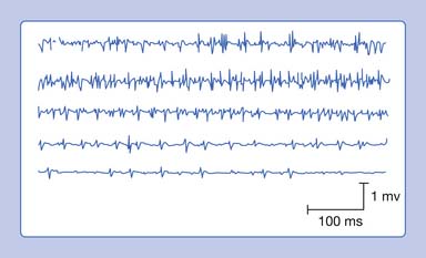
A needle recording electrode placed into a cramping muscle shows multiple motor units firing synchronously between 40 and 60 Hz, and occasionally reaching 200 to 300 Hz (Figure 9-23). A large portion of the muscle is simultaneously involved in a cramp, as opposed to the asynchronous excitation of motor units during voluntary activation. Cramps are believed to arise from a peripheral portion of the motor unit. A cramp that results in a taut muscle with electrical silence is the physiologic contracture seen in McArdle disease.
Multiplet Discharges
A clinical syndrome manifested by spontaneous muscle twitching, cramps, and carpopedal spasm is known as tetany.14 This entity usually results from peripheral and/or central nervous system irritability associated with systemic alkalosis, hypocalcemia, hyperkalemia, hypomagnesemia, or local ischemia. Clinically, one can induce tetany by tapping the facial nerve (Chvostek’s sign), the peroneal nerve at the fibular head (peroneal sign), and inducing limb ischemia (Trousseau’s sign).
In the above conditions, characteristic motor unit potentials can be observed. A single motor unit potential might fire rather rapidly, with an interdischarge interval of 2 to 20 ms. If the motor unit fires twice, it is referred to as a doublet; three times denotes a triplet; and more than three firings is called a multiplet (Figure 9-24). These potentials can be seen after voluntary contraction, or can be observed spontaneously from the induction maneuvers noted above (Chvostek’s sign or Trousseau’s sign), in which MUAPs can fire in long trains or short bursts of 5 to 30 Hz (tetany). Motor units with an interdischarge interval of 20 to 80 ms are called “paired discharges” but can arise in similar states, as previously described.
Nerve Injury Classification
Seddon’s Classification
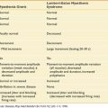
The degree to which a nerve is damaged has obvious implications with respect to its present function and potential for recovery. There are essentially two general classification systems.39,43 One classification is that of Seddon, and considers neural injury from the perspective of a combination of functional status and histologic appearance. In Seddon’s scheme, there are three degrees or stages of injury to consider: neurapraxia, axonotmesis, and neurotmesis (Table 9-1).

Axonotmesis
The second degree of neural insult in Seddon’s classification is axonotmesis, which is a specific type of nerve injury where only the axon is physically disrupted, with preservation of the enveloping endoneurial and other supporting connective tissue structures (perineurium and epineurium). Compression of a profound nature and traction on the nerve are typical lesion etiologies. Once the axon has been disrupted, the characteristic changes of wallerian degeneration occur. The fact that the endoneurium remains intact is a very important aspect of this type of injury. A preserved endoneurium implies that once the remnants of the degenerated nerve have been removed by phagocytosis, the regenerating axon simply has to follow its original course directly back to the appropriate end organ. A good prognosis can be expected when neural damage results only in axonotmesis.
Sunderland’s Classification
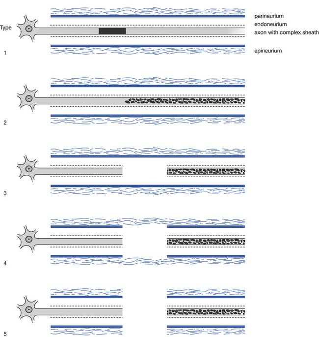
A second popular and somewhat more detailed classification is that proposed and subsequently modified by Sunderland. This classification of nerve injury is based on the results of trauma with respect to the axon and its supporting connective tissue structures. Basically, Sunderland’s classification is divided into five types of injury, based exclusively on which connective tissue components are disrupted (Figure 9-25). Type 1 injury corresponds to Seddon’s designation of neurapraxia. Seddon’s axonotmesis is subdivided by Sunderland into three forms of neural insult (types 2 through 4). A type 2 injury involves loss of axonal continuity with preservation of all supporting neural structures, including the endoneurium (this closely corresponds to Seddon’s axonotmesis). Type 3 and 4 injuries result in progressively more neural disruption. Sunderland’s type 5 injury corresponds to Seddon’s neurotmesis (complete neural disruption).
Instrumentation
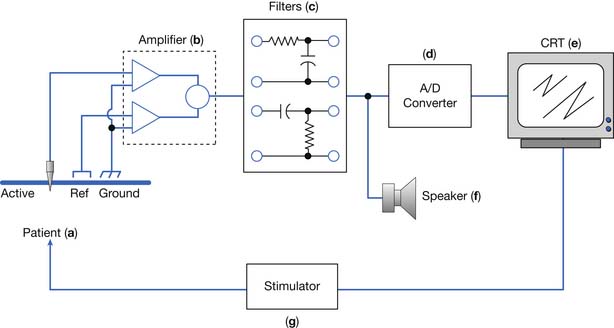
An electrodiagnostic instrument actually comprises many separate components, of which the electrodes, amplifier, filters, sound, and stimulator are discussed in this chapter. Practitioners of electrodiagnostic medicine are urged to gain a thorough understanding of instrumentation principles and all the instrument’s subcomponents (Figure 9-26).17,18,41
Electrodes
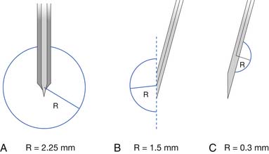
Two commonly used needle recording electrodes are monopolar and concentric (Figure 9-27). The monopolar needle is a solid, stainless steel shaft coated completely with Teflon except for the bare metal tip. It is this bare metal tip that acts as the recording surface. The needle is typically 12 to 75 mm in length and 0.3 to 0.5 mm in diameter, with a recording surface of 0.15 to 0.6 mm2. Separate reference and ground electrodes are required. The concentric needle electrode is a hollow, stainless steel hypodermic needle with a central platinum or Nichrome-silver wire about 0.1 mm in diameter, surrounded by epoxy resin acting as an insulating material from the surrounding cannula. The cannula has a similar length and diameter to that of the monopolar needle. A separate ground is required, but the cannula serves as the reference electrode.
There has been considerable discussion about the merits of each of these electrodes compared with the other. Both electrodes have advantages and disadvantages depending on the clinical circumstances. Monopolar needle electrodes have a wider recording territory and a distant reference, which makes the recording more “noisy” with respect to distant activity and interference. On the other hand, the Teflon coating probably reduces patient discomfort depending on technique. The concentric needle electrode has the active and reference electrodes close together, making them electrically quieter than monopolar needles. Concentric electrodes typically cause more patient discomfort, but again, this is likely technique dependent. Concentric needle electrodes yield the following as compared with monopolar needle electrodes: smaller potential amplitudes, possibly fewer phases, comparable durations, and less distant motor unit activity. The introduction of commercially available, disposable monopolar and concentric needle electrodes has eliminated such worries as Teflon peeling back on the monopolar needles, and hook formation on the tip of the concentric needle electrodes. The quality of disposable needle electrodes has improved, eliminating the need to use nondisposable needle electrodes. If electrodes are reused, they should be properly sterilized with presoaking in sodium hypochlorite and steam autoclaving.14 There are concerns about the possibility of spreading prion disease using sterilized, reusable needles.37 Documentation of this, however, is lacking.
Single-fiber electrodes are essentially modified concentric needle electrodes. A small, 25-μm recording port is placed opposite the electrode’s bevel and several millimeters from the tip. This makes this special electrode capable of recording the electrical activity from a single muscle fiber. The uptake area for this electrode is approximately 300 μm (see Figure 9-27). Recent studies show comparable jitter values comparing disposable concentric needles and single-fiber electrodes.32
Amplifier
Biologic signals range in size from microvolts to millivolts, thereby requiring significant amplification before being analyzed. An amplifier is simply a device with the ability to magnify the desired signals and minimize unwanted signals or noise. Amplification is expressed as gain or sensitivity. Gain is a ratio of the signal’s output divided by the input. For example, an output of 1 V for an input of 10 mV implies that the amplifier has a gain factor of 100,000 (output/input= 1V/0.00001V= 100,000). Sensitivity is the ratio of the input voltage to the size of deflection on the CRT, and is usually measured in centimeters. For example, an amplifier that produces a 1-cm deflection for an input of 10 mV has a sensitivity of 10 mV/cm or 10 mV/division. The sensitivity or gain setting used is important because it can influence the onset latency. Increasing the sensitivity for a given waveform results in the instrument displaying the potential’s initial departure from baseline earlier in time, because progressively earlier and hence smaller baseline deviations can now be observed.
Filters
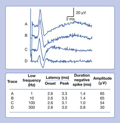
In our example, a recorded median SNAP and CMAP are sequentially distorted by altering the low- and high-frequency filter settings. Let us begin with an arbitrary low-frequency filter setting of 1 Hz and a high-frequency filter cutoff of 10,000 Hz. Sequentially elevating the low-frequency filter from 1 to 10 Hz, 100 Hz, and finally 300 Hz, while maintaining a high-frequency filter at 10,000 Hz, results in characteristic waveform distortions (Figure 9-28). The onset latency does not change, the peak latency decreases, amplitude is serially reduced, and the total potential duration decreases. Also, an additional phase is created. The use of sequentially higher low-frequency filter settings removes progressively more low frequencies from the SNAP. In other words, the remaining potential now has a predominance of high frequencies in it as compared with the original potential. The onset of the potential remains unaltered because it is a quick departure from baseline and is not influenced by an alteration in the low-frequency content of the waveform. The remainder of the potential, however, is influenced by the now predominant high-frequency subcomponent waveforms. By taking out the low frequencies, the amplitude declines as subcomponent waveforms are removed. Clearly, the waveform’s magnitude could not possibly increase because we are taking out part of its content. Further, the remainder of the waveform is shifted to an earlier time of occurrence because of the high frequencies remaining in the SNAP. Because comparatively high frequencies occur sooner in time, it is logical that all the waveform shifts toward the potential’s stationary onset, producing decreases in its peak latency, negative spike duration, and total duration. A third phase is created as the potential begins to appear more like a sine wave as the higher frequencies begin to emerge. Remember, high frequencies have more phases per unit time. A similar but more dramatic occurrence is noted for the CMAP, because it comprises comparatively more low frequencies than a SNAP does.
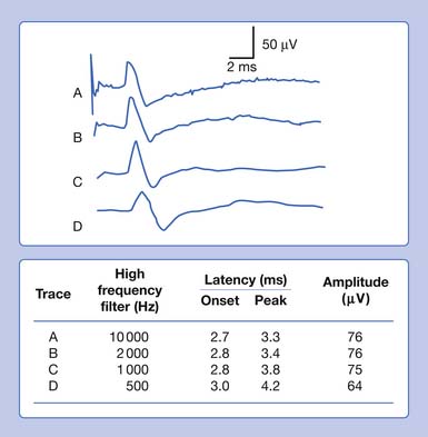
Eliminating high frequencies results in a somewhat different set of alterations. Because we are removing waveforms from the total potential, a reduction in amplitude can be anticipated. Because the SNAP is now biased toward a potential with more low frequencies, it takes longer to occur in time. This results in a delay of both the onset and the peak latencies (Figure 9-29). Lowering the high-frequency filter while maintaining a constant low-frequency filter results in a waveform with a comparatively smaller amplitude, longer onset latency, and longer peak latency, as well as longer overall duration. Similar findings can be observed for a CMAP.
There are no universally agreed filter settings for any electrodiagnostic medicine procedure. Arriving at optimal filter settings is highly empiric. The high- and low-frequency filters are lowered and raised, respectively, until waveform distortions are observed. The filters are then expanded until no waveform changes are noted. The goal is to include the major components of the waveforms while eliminating undesired signals or noise. The most important factor is to reproduce all filter settings originally described by those investigators whose reference data are being used (Table 9-2).
| Procedure | Low Frequency (Hz) | High Frequency (Hz) |
|---|---|---|
| Nerve conduction velocity (motor) | 2-10 | 10,000 |
| Nerve conduction velocity (sensory) | 2-10 | 2000 |
| Needle electromyography (routine) | 20-30 | 10,000 |
| Needle electromyography (quantitative) | 2-5 | 10,000 |
| Single-fiber electromyography | 500-1000 | 10,000-20,000 |
| Somatosensory evoked potential | 1-10 | 500-3000 |
From Dumitru D, Walsh NE. Practical instrumentation and common sources of error, Am J Phys Med Rehabil 67:55-65, 1988, with permission.
Stimulator
Two different types of stimulators are commercially available: constant current and constant voltage. For both types of devices, neural tissue is activated under the cathode (negative pole) while the anode (positive pole) completes the stimulating circuit. A constant current stimulator effectively delivers the desired current output for each stimulus irrespective of the resistance between the skin and cathode or anode. This is accomplished by varying the voltage or current driving force as is necessitated by any alterations in the skin-stimulator interface’s resistance. Similarly, a constant voltage stimulator is designed to deliver the same voltage with each stimulus, even if the resistance between the skin and stimulator changes. A compensatory increase or decrease in current is provided so as to maintain the same voltage level. In short, a constant current stimulator is effectively a variable voltage stimulator, while a constant voltage stimulator is a variable current stimulator. Both stimulators are acceptable for most purposes. The constant current stimulator is preferred when the same current must be delivered for each stimulus in clinical situations requiring quantification of current delivery, such as in somatosensory evoked potentials, research, or evaluating side-to-side stimulation thresholds during facial nerve excitability testing.
1. Albers J.W., Allen A.A., Bastron J.D., et al. Limb myokymia. Muscle Nerve. 1981;4:494-504.
2. Baer R.D., Johnson E.W. Motor nerve conduction velocities in normal children. Arch Phys Med Rehabil. 1965;46:698-704.
3. Bolton C.F., Carter K.M. Human sensory nerve compound action potential amplitude: variation with sex and finger circumference. J Neurol Neurosurg Psychiatry. 1980;43:925-928.
4. Brown W.F. The physiological and technical basis of electromyography. Boston: Butterworth; 1984.
5. Buchthal F. Fibrillations: clinical electrophysiology. In: Culp W.J., Ochoa J., editors. Abnormal nerves and muscle generators. New York: Oxford University Press, 1982.
6. Buchthal F., Guld C., Rosenfalck P. Multielectrode study of the territory of a motor unit. Acta Physiol Scand. 1957;39:83-104.
7. Buchthal F., Guld C., Rosenfalck P. Volume conduction of the spike of the motor unit potential investigated with a new type of multielectrode. Acta Physiol Scand. 1957;38:331-354.
8. Buchthal F., Rosenfalck A. Evoked action potentials and conduction velocity in human sensory nerves. Brain Res. 1966;3:1-122.
9. Campbell W.W., Ward L.C., Swift T.R. Nerve conduction velocity varies inversely with height. Muscle Nerve. 1981;4:520-523.
10. Cummins K.L., Dorfman L.J. Nerve fiber conduction velocity distributions: studies of normal and diabetic human nerves. Ann Neurol. 1981;9:67-74.
11. Daube J.A. AAEM minimonograph #11: needle examination in electromyography. Rochester: AAEM; 1979.
12. Daube J.R., Rubin D.I. Needle electromyography. Muscle Nerve. 2009;39:244-270.
13. Dumitru D. Volume conduction: theory and application. In: Dumitru D., editor. Physical medicine and rehabilitation state of the art reviews: clinical electrophysiology. Philadelphia: Hanley & Belfus, 1989.
14. Dumitru D., Amato A.A., Zwarts M.J. Electrodiagnostic medicine, ed 2. Philadelphia: Hanley & Belfus; 2002.
15. Dumitru D., Martinez C.T. Propagated insertional activity: a model of positive sharp wave generation. Muscle Nerve. 2006;34:457-462.
16. Dumitru D., Santa Maria D.L. Positive sharp wave origin: evidence supporting the electrode initiation hypothesis. Muscle Nerve. 2007;36:349-356.
17. Dumitru D., Walsh N.E. Practical instrumentation and common sources of error. Am J Phys Med Rehabil. 1988;67:55-65.
18. Dumitru D., Walsh N.E. Electrophysiologic instrumentation. In: Dumitru D., editor. Physical medicine and rehabilitation state of the art reviews: clinical electrophysiology. Philadelphia: Hanley & Belfus, 1989.
19. Falco F.J.E., Hennessey W.J., Braddom R.L., et al. Standardized nerve conduction studies in the upper limb of the healthy elderly. Am J Phys Med Rehabil. 1992;71:263-271.
20. Falco F.J.E., Hennessey W.J., Goldberg G., et al. H reflex latency in the healthy elderly. Muscle Nerve. 1994;17:161-167.
21. Halar E.M., DeLisa J.A. Peroneal nerve conduction velocity: the importance of temperature control. Arch Phys Med Rehabil. 1981;62:439-443.
22. Halar E.M., DeLisa J.A., Brozovich F.V. Nerve conduction velocity: relationship of skin, subcutaneous and intramuscular temperatures. Arch Phys Med Rehabil. 1980;61:199-203.
23. Halar E.M., DeLisa J.A., Soine T.L. Nerve conduction studies in upper extremities: skin temperature corrections. Arch Phys Med Rehabil. 1983;64:412-416.
24. Henrikson J.D. Conduction velocity of motor nerves in normal subjects and patients with neuromuscular disorders [thesis]. Minneapolis: University of Minnesota; 1956.
25. Hille B., et al. Introduction to physiology of excitable cells. In Patton H.D., Fuchs A.F., Hille B., editors: Textbook of physiology, ed 21, Philadelphia: WB Saunders, 1989.
26. Hodgkin A.L., Huxley A.F. A quantitative description of membrane current and its application to conduction and excitation in nerve. J Physiol. 1952;117:500-544.
27. Hodgkin A.L., Katz B. The effect of temperature on the electrical activity of the giant axon of the squid. J Physiol. 1949;109:240-249.
28. Jewett D.L., Rayner M.D. Basic concepts of neuronal function. Boston: Little Brown; 1984.
29. Johnson E.W., Olsen K.J. Clinical value of motor nerve conduction velocity determination. JAMA. 1960;172:2030-2035.
30. Katz B. Nerve, muscle, and synapse. New York: McGraw-Hill; 1966.
31. Koester J. Resting membrane potential and action potential. In Kandel E.R., Schwartz J.H., editors: Principles of neural science, ed 2, New York: Elsevier, 1985.
32. Kouyoumdjian J.A., Stålberg E.V. Concentric needle single fiber electromyography: comparative jitter on voluntary-activated and stimulated extensor digitorum communis. Clin Neurophysiol. 2008;119:1614-1618.
33. Lang A.H., Forsstrom J., Bjorkqvist S.E., et al. Statistical variation of nerve conduction velocity: an analysis in normal subjects and uraemic patients. J Neurol Sci. 1977;33:229-241.
34. Layzer R.B., Rowland L.P. Cramps. N Engl J Med. 1971;285:30-31.
35. Lundborg G. Nerve injury and repair. Edinburgh: Churchill Livingstone; 1988.
36. Oh S.J. Clinical electromyography: nerve conduction studies, ed 2. Baltimore: Williams & Wilkins; 1993.
37. Rosted P., Jørgensen V.K. Reusable acupuncture needles are a potential risk for transmitting prion disease. Acupunct Med. 2001;19:71-72.
38. Schoepfle G.M., Erlanger J. The action of temperature on the excitability, spike height and configuration, and the refractory period observed in the responses of single medullated nerve fibers. Am J Physiol. 1941;134:694-704.
39. Seddon H. Three types of nerve injury. Brain. 1943;66:237-288.
40. Soudmand R., Ward L.C., Swift T.R. Effect of height on nerve conduction velocity. Neurology. 1982;32:407-410.
41. Stolov W. Instrumentation and measurement in electrodiagnosis. Minimonograph #16. Rochester: American Association of Electrodiagnostic Medicine; 1981.
42. Streib E.W. AAEM minimonograph #27: differential diagnosis of myotonic syndromes. Muscle Nerve. 1987;10:603-615.
43. Sunderland S. A classification of peripheral nerve injuries producing loss of function. Brain. 1951;74:491-516.
44. Sunderland S. Nerve injuries and their repair: a critical appraisal. Edinburgh: Churchill Livingstone; 1991.
45. Thesleff S. Fibrillation in denervated mammalian muscle. In: Culp W.J., Ochoa J., editors. Abnormal nerve and muscle as impulse generators. New York: Oxford University Press, 1982.
46. Trojaborg W. Motor nerve conduction velocities in normal subjects with particular reference to the conduction in proximal and distal segments of median and ulnar nerve. Electroencephalogr Clin Neurophysiol. 1964;17:314-321.
47. Waxman S.G. Action potential propagation and conduction velocity: new perspectives and questions. Trends Neurosci. 1983;6:157-161.
48. Waxman S.G., Foster R.E. Ionic channel distribution and heterogeneity of the axon membrane in myelinated fibers. Brain Res Rev. 1980;2:205-234.