[level-membership-for-anesthesiology-category]
15 Electrocardiographic Monitoring
As late as 1970, the electrocardiographic monitor was not considered an integral part of monitoring strategies in the perioperative period. As a matter of fact, luminaries in the specialty regarded the use of ECG monitoring as “questionable value because of possible iatrogenic problems.” Concern also was expressed that anesthesiologists’ attention would be diverted from the patient.1 Currently, monitoring the ECG is a fundamental standard of monitoring of the American Society of Anesthesiologists.2 Despite the introduction of more sophisticated cardiovascular monitors such as the pulmonary artery catheter and echocardiography, the electrocardiogram (ECG; coupled with blood pressure measurement) serves as the foundation for guiding cardiovascular therapeutic interventions in the majority of anesthetics.3 It is indispensable for diagnosing arrhythmias, acute coronary syndromes, electrolyte abnormalities, (particularly of serum potassium and calcium), and some forms of genetically mediated electrical or structural cardiac abnormalities (e.g., Brugada syndrome; Table 15-1).4
TABLE 15-1 Basic Clinical Information Available from Electrocardiography
| Anatomy or Morphology |
| Physiology |
One of the most important changes in electrocardiography that has occurred recently is the widespread use of computerized systems for recording ECGs. Bedside units are capable of recording diagnostic quality 12-lead ECGs that can be transmitted over a hospital network, for storage and retrieval. Most of the ECGs in the United States are recorded by digital, automated devices, equipped with software, which can measure ECG intervals and amplitudes and provide a virtually instantaneous interpretation. However, different automated systems may have different technical specifications that can result in significant differences in the measurement of amplitudes, intervals, and diagnostic statements.5,6 The diagnostic specificity and sensitivity of the ECG to diagnose a particular abnormality also are not consistent. For example, finite limits are defined by the relation between sensitivity and specificity (usually inversely related) for detecting obstructive coronary artery disease (CAD). During exercise testing, the 12-lead ECG has a mean sensitivity of only 68% and a specificity of 77%.7,8 The resting 12-lead ECG is even less sensitive and specific.8 More complex ECG modalities are likely to improve its utility in the future (high-frequency QRS signal averaging). In this chapter, the theory and the operating characteristics of ECG hardware used in the perioperative period are presented to facilitate proper use and interpretation of monitoring data.
Historical perspective
An extensive review of the history of electrocardiography is beyond the scope of this chapter. However, several excellent reviews were published in honor of the centennial of the first recording of the human ECG.9–14 Willem Einthoven is universally considered the father of electrocardiography (for which he won the 1924 Nobel Prize for Medicine/Physiology). Many of the basic clinical abnormalities in electrocardio-graphy were first described using the string galvanometer (e.g., bundle branch block, delta waves, ST-T changes with angina). It was used until the 1930s, when it was replaced by a system using vacuum tube amplifiers and a cathode ray oscilloscope. With advancements in electrical engineering technology, the devices became more compact, portable, and user friendly. In the 1950s, a portable direct-writing ECG cart was introduced. The first analog-to-digital (A/D) conversion systems for the ECG were introduced in the early 1960s, although their off-line use was impractical and restricted until the late 1970s. In the 1980s, microcomputer technology became widely available and is now standard for all diagnostic and monitoring systems. Further improvements in hardware and software design led to the development of automated ST-analysis algorithms and their use in routine clinical practice.
Basic electrophysiology and electrical anatomy of the heart
The ECG is the final result of a complex series of physiologic and technologic processes.15 Physiologically, the ECG reflects differences in transmembrane voltages in myocardial cells that occur during depolarization and repolarization within each cycle. Ionic currents are generated because of ionic fluxes across cell membranes in myocardial cells during depolarization and repolarization. The cardiac cells are con tiguous and electrically connected by ion channels (gap junctions), which allows the ion current to pass through the cells and spread depolarization.16 Thus, the membrane potential changes in the heart can be considered a single depolarization that propagates through the whole heart, assuming different forms along the way.16 The pattern and sequence of depolarization that occur in the heart are depicted in Figure 15-1. There are many different types and subtypes of ion channels that are involved in the synchronized generation of electrical activity in the heart. Of note are the sodium, potassium, calcium, and chloride channels.15–17 Detailed discussion of these channels is beyond the scope of this chapter.
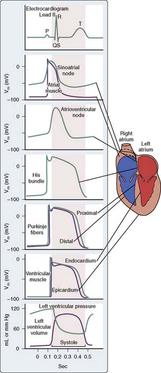
At any point in time, the electrical activity of the heart is composed of differently directed electrical forces. However, these currents are synchronized by cardiac activation and recovery sequences to generate a cardiac electrical field in and around the heart that varies with time during the cardiac cycle. This cardiac electrical field passes through various internal structures such as lungs, blood, and skeletal muscles. The currents reaching the skin are then detected by the electrodes that are placed in specific locations on the body and uniquely configured to produce different ECG patterns or waveforms. Direction and strength of a lead vector depend on the geometry of the body and on the varying electric impedances of the tissues in the torso.18,19 As expected, placement of electrodes on the torso is distinct from direct placement on the heart because the localized signal strength that occurs with direct electrode contact is markedly attenuated and altered by torso inhomogeneities, which include thoracic tissue boundaries and variations in impedance. The standard 12-lead ECG records potential differences (represented as change of voltage over time) between prescribed sites on the body surface that vary during the cardiac cycle.4
The first deflection noted on the ECG is caused by atrial depolarization and is called the P wave. Although the depolarization of the sinoatrial node precedes the atrial depolarization (see Figure 15-1), the potential from these pacemaker cells are too small to be detected on the surface ECG. The width of the P wave reflects the time taken for the wave of depolarization to spread over both the right and left atria. In comparison with the ventricular action potential, the atrial action potential is narrower and has a less prominent plateau. The duration of atrial contraction is, thus, shorter, which permits another action potential to occur sooner and makes atria prone to a very high rate (atrial flutter). The repolarization atrial wave rarely is seen in a normal ECG because it is buried in the much larger QRS wave.
The ECG returns to its baseline between the end of atrial depolarization and the commencement of the QRS complex, which is the start of the QRS ventricular depolarization. This interval is called the PR interval. Though this period may seem electrically silent, it is a time of significant electrical activity. During this period, the wave of depolarization that started in the sinoatrial node is propagated through the AV node, the AV bundle, right and left bundle branches, and Purkinje fibers (see Figure 15-1).
The QRS wave is followed by a period when the ECG returns to the baseline and is called the ST segment. It is a time when the ventricle is completely depolarized and is represented by phase 2 of the action potential (see Figure 15-1). Even though the ventricles are depolarized, the ECG does not record any positive or negative waveforms because the whole ventricles are depolarized and there is no potential difference between sites. The ECG does not measure absolute levels of membrane potential but only records the potential differences.15 The same explanation also holds true for the T-P segment, which represents a time when the ventricles are fully repolarized; hence no significant potential difference is recorded on a surface ECG.
Sometimes small undulations can be seen after T waves but before P waves. These are called U waves and are thought to be generated by M cells, which are specialized midmyocardial cells with prolonged action potentials.15
Technical aspects of the electrocardiogram
Most clinicians assume that the ECG is a relatively simple technical device. However, an extensive amount of advanced electrical theory underlies both the recording and display of the ECG signal. Digital signal processing (DSP) is now used universally, and the average ECG unit incorporates several microprocessors. Anesthesiologists should familiarize themselves with the theory behind ECG acquisition to maximize rational clinical application and appreciate its clinical limitations. In this section, the basics of electrocardiography are presented, briefly considering the major components that are involved in the faithful rendition of the surface ECG, working from the skin and electrodes progressively to the final output on the screen. The reader is referred to a number of technical reviews for more detail.4,5,12,20–23
Processing of the ECG occurs in a series of steps as shown in Figure 15-2.4 These steps include (1) signal acquisition, including filtering; (2) data transformation, or rendition of data for further processing, including finding the complexes, classification of the complexes into “dominant” and “nondominant” (ectopic) types, and formation of an average or median complex for each lead; (3) waveform recognition, which is the process for identification of the onset and offset of the diagnostic waves; (4) feature extraction, which is the measurement of intervals and amplitudes; and (5) for the bedside 12-lead ECG machines, diagnostic classification.4 Diagnostic classification may be heuristic (i.e., deterministic, or based on experience-based rules) or statistical in approach.24
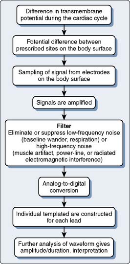
Figure 15-2 Schematic representation of the processes resulting in recording of the electrocardiogram.

Signal Acquisition and Power Spectrum of the Electrocardiogram
It is relevant to consider an electrocardiographic signal in terms of its amplitude (or voltage) and its frequency components (generally called its phase) to appreciate ECG signal acquisition. Voltage considerations differ depending on the signal source. Surface recording involves amplification of smaller voltages (on the order of 1 mV) than recording sites closer to the heart beneath the electrically resistant layers of the skin (e.g., endocardial, esophageal, and intratracheal leads). The “power spectrum” of the ECG (Figure 15-3) is derived by Fourier transformation, in which a periodic waveform is mathematically decomposed to its harmonic components (sine waves of various amplitudes and frequencies). The fundamental frequency for the QRS complex at the body surface is approximately 10 Hz, and most of the diagnostic information is contained below 100 Hz in adults. Spectra representing some of the major sources of artifact must be eliminated during the processing and amplification of the QRS complex.22 The frequency of each of these components can be equated to the slope of the component signal.6 The R wave with its steep slope is a high-frequency component (100 Hz), whereas P and T waves have lesser slopes and are lower in frequency (1 to 2 Hz). The ST segment has the lowest frequency, not much different from the “underlying” electrical (i.e., isoelectric) baseline of the ECG. Before the introduction of DSP, accurately displaying the ST segment presented significant technical problems, particularly in operating room and intensive care unit bedside monitoring units. Although the overall frequency spectrum of the QRS complex does not appear to exceed 40 Hz, many components of the QRS complex, particularly the R wave, can exceed 100 Hz. The American Heart Association (AHA) recommends a bandwidth of 0.05 to 100 Hz for monitoring and detection of myocardial ischemia.4 Very-high-frequency signals of particular clinical significance are pacemaker spikes. Their short duration and high amplitude present technical challenges for proper recognition and rejection to allow accurate determination of the heart rate. The frequencies of greatest importance for optimal ECG processing are presented in Table 15-2.5
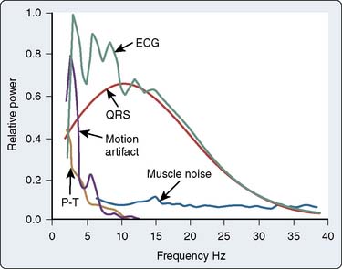
TABLE 15-2 Range of Signal Frequencies Included in Different Phases of Processing in an Electrocardiographic Monitor
| Processing | Frequency Range |
|---|---|
| Display | 0.5 (or 0.05)–40 Hz |
| QRS detection | 5–30 Hz |
| Arrhythmia detection | 0.05–60 Hz |
| ST-segment monitoring | 0.05–60 Hz |
| Pacemaker detection | 1.5–5 kHz |

Digital Signal Processing of the Electrocardiogram
Computerized ECG processing has been adapted to all major clinical applications of the ECG. The earliest application of A/D signal processing occurred during exercise tolerance testing, when significant motion artifact and electromyographic noise make acquisition of a “clean” ECG signal difficult. Outside of the exercise treadmill laboratory, computer processing allows automated analysis of the diagnostic 12-lead ECG.25 The reader is referred elsewhere for more detailed discussions of this technology, and to the reports of the scientific council of the AHA on standardization and specifications for automated ECG and bedside monitors.4,25–28
Processing of the ECG signal by a digital electrocardiograph involves initial sampling of the signal from electrodes on the body surface. Nearly all current-generation ECG machines convert the analog ECG signal to digital form before further processing. The foundation of DSP is the A/D converter, which samples the incoming “continuous” analog signal (characterized by variable amplitude or voltage over time) at a very rapid rate, converting the sampled voltage into binary numbers, each of which has a precise time index or sequence. Greater sampling rates (≥ 10,000 to 15,000/sec), which are typically less than 0.5 millisecond in duration help detect pacemaker output reliably. Several technical recommendations regarding low-frequency filtering and high-frequency filtering recently have been published by the AHA.4

Formation of a Representative Single-Lead Complex
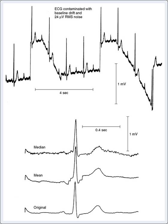
QRS waveform amplitudes and durations are subject to beat-to-beat variability and to respiratory variability between beats. Digital ECGs can adjust for respiratory variability and decrease beat-to-beat noise to improve the measurement precision in individual leads by forming a representative complex for each lead. Signal averaging is a critical component of this process. Noise is reduced using this technique proportionate by the square root of the number of beats averaged.4 Thus, a 10-fold reduction in noise is accomplished by averaging only 100 beats. Automated measurements are made from these representative templates, not from measurement of individual complexes. Average complex templates are formed from the average amplitude of each digital sampling point for selected complexes. Median complex templates are formed from the median amplitude at each digital sampling point. As a result, measurement accuracy is strongly dependent on the fidelity with which representative templates are formed. Because of the proprietary nature of this technology (the specific algorithms used are patented), the method used may vary by manufacturer. Consequently, the processed QRS complexes may vary in the “quality” of representation (i.e., if noise or aberrant beats are averaged into the complex, it will vary from the raw analog complex). The averaging process involves comparison of the voltages at a particular time point between the incoming complex and the template. Although the easiest method is to use the mean difference between voltages to update the “template,” the most accurate method is to use the median (because it is less affected by outliers, such as aberrant beats or other signals that have escaped QRS matching)4 (Figure 15-4).
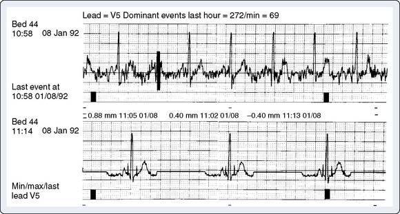
A feature incorporated into most monitors is a visual trend line from which deviations in the position of the ST segment can be rapidly detected, which can aid online detection of ischemia. In addition, nearly all monitors display on-screen numerical values for the position of the ST segment used for ischemia detection (generally 60 to 80 milliseconds after the J point), although the specific fiducial point (based on heart rate) used usually can be adjusted by the clinician (Figure 15-5).

History and Description of the 12-Lead System
Where and how ECG electrodes are placed on the body are critical determinants of the morphology of the ECG signal. Lead systems have been developed based on theoretical considerations and references to anatomic landmarks that facilitate consistency between individuals (e.g., standard 12-lead system). Einthoven established electrocardiography using three extremities as references: the left arm, right arm, and left leg. He recorded the difference in potential between the left arm and right arm (lead I), between the left leg and right arm (lead II), and between the left leg and left arm (lead III) (Figure 15-6). Because the signals recorded were differences between two electrodes, these leads were called bipolar. The right leg served only as a reference electrode. Because Kirchoff’s loop equation states that the sum of the three voltage differential pairs must equal zero, the sum of leads I and III must equal lead II.21 The positive or negative polarity of each of the limbs was chosen by Einthoven to result in positive deflections of most of the waveforms and has no innate physiologic significance. He postulated that the three limbs defined an imaginary equilateral triangle with the heart at its center. Wilson refined and introduced the precordial leads into clinical practice. To implement these leads, he postulated a mechanism whereby the absolute level of electrical potential could be measured at the site of the exploring precordial electrode (the positive electrode). A negative pole with zero potential was formed by joining the three limb electrodes in a resistive network in which equally weighted signals cancel each other out. He called this the “central terminal,” and in a fashion similar to Einthoven’s vector concepts, he postulated it was located at the electrical center of the heart, representing the mean electrical potential of the body throughout the cardiac cycle. He described three additional limb leads (aVL, aVR, and aVF; Figure 15-7). These leads measured new vectors of activation, and in this way, the hexaxial reference system for determination of electrical axis was established. He subsequently introduced the six unipolar precordial V leads in 1935 (see Figure 15-6).29 Six electrodes are placed on the chest in the following locations: V1, fourth intercostal space at the right sternal border; V2, fourth intercostal space at the left sternal border; V3, midway between V2 and V4; V4, fifth intercostal space in the midclavicular line; V5, in the horizontal plane of V4 at the anterior axillary line, or if the anterior axillary line is ambiguous, midway between V4 and V6; and V6, in the horizontal plane of V4 at the midaxillary line4 (see Figure 15-6).
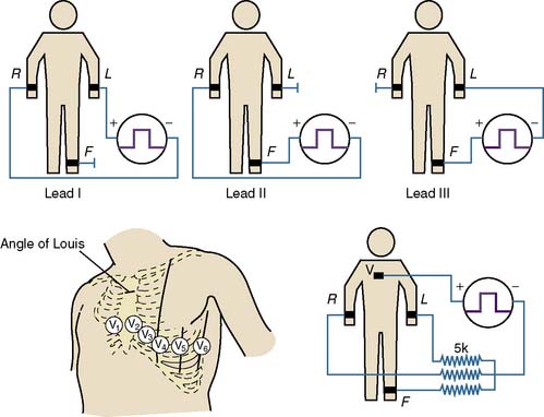
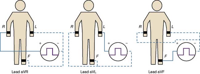
Clinical application of the unipolar limb leads was limited because of their significantly smaller amplitude relative to the bipolar limb leads from which they were derived. They were not clinically applied until Goldberger augmented their amplitude (by a factor of 1.5) by severing the connection between the central terminal and the lead extremity being studied (which he called “augmented limb leads”) in 1942. The limb leads, the precordial leads, and the augmented unipolar limb leads form what was accepted by the AHA as the conventional 12-lead ECG system.30 Einthoven’s law indicates that any one of the standard limb leads can be mathematically derived from the other two limb leads. Therefore, the “standard” 12-lead ECG actually contains eight independent pieces of information: two measured potential differences from which the four remaining limb leads can be calculated and the six independent precordial leads.4 In essence, all leads are effectively “bipolar,” and the differentiation between “bipolar” and “unipolar” in the description of the standard limb leads, the augmented limb leads, and the precordial leads is discouraged in the most recent statement by the AHA.4


Intrinsic and Extrinsic Electrocardiogram Artifact
Skin Impedance
Motion artifact and “baseline wander” result from several causes. Intrinsic to the body are electrical potentials generated by the skin.31 Skin impedance has been shown to vary at different skin sites.
Motor Activity
Another major physiologic source of artifact is electromyographic noise produced by motor activity, either voluntary (i.e., during treadmill testing or ambulatory ST-segment monitoring) or involuntary (i.e., shivering or Parkinsonian tremor). Electromyographic noise is similar in amplitude to the ECG but is generally of considerably higher frequency. Because it is a random signal, in contrast with the regular repetitive ECG, it is amenable to significant attenuation using routine DSP techniques (Figure 15-8).32
Extrinsic
There are also extrinsic or nonphysiologic causes of artifact. An important one is called common-mode rejection. The ECG signal is recorded as the difference in potential between two electrodes and is technically a differential signal. The body is not at absolute ground potential, which is why the right leg lead is used as a reference electrode.22 This higher potential (over that of an absolute ground to earth) is called common-mode potential because it is common to both electrode inputs to the differential amplifier used to amplify the ECG signal. Common-mode potential must be rejected or it may alter the ECG signal.
Electrical Power-line Interference
Electrical power-line interference (60 Hz) is a common environmental problem. Power lines and other electrical devices radiate energy that can enter the monitor by poor electrode contact or cracked or poorly shielded lead cables. Interference can also be induced electromagnetically as these signals radiate through the loop formed by the body, lead cables, and monitor.31 This type of interference can be reduced by twisting the lead cables together (reducing the loop area) or by minimizing the distance between the lead cables. In newer diagnostic ECG machines, A/D signal conversion occurs in an acquisition module close to the patient, which effectively reduces the length of the lead cables and the amount of signal induction possible. A line frequency “notch” filter is often used to remove 60-Hz noise. Other means of mathematical manipulation and processing also can remove 60-Hz noise.33
Electrocautery
Electrocautery units generate radiofrequency currents at very high frequencies (800 to 2000 kHz) and high voltages (1 kV, which is 100 times greater than the ECG signal). Older units used a modulation frequency of 60 Hz, which spread substantial electrical noise into the QRS frequency range of the ECG signal. Newer units use a modulation frequency of 20 kHz, minimizing this problem.5 To minimize electrocautery artifact, place the right leg reference electrode as close as possible to the return plate and plug the ECG monitor into a different power outlet from the electrosurgical unit.

Clinical Sources of Artifact
Clinical devices with which the patient is in physical contact, particularly via plastic tubing, may at times cause clinically significant ECG artifact.34–37 Although the exact mechanism is uncertain, two leading explanations are either a piezoelectric effect caused by mechanical deformation of the plastic or buildup of static electricity between two dissimilar materials, especially those in motion (as in the case of cardiopulmonary bypass [CPB] tubing and the roller pump head described later). In this scenario, the electricity generated in the pump flows into the patient via the tubing and is picked up by the electrodes. This artifact is not related to the electricity used to power the CPB pump because it has been reproduced by manually turning the pump heads.
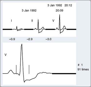
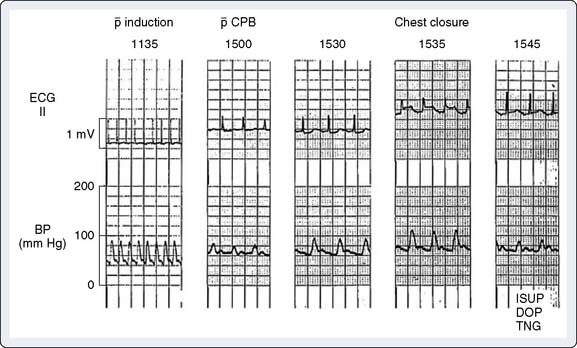
Although ECG interference during CPB has been recognized for many years, Khambatta et al36 were the first to document it in the literature. It is manifested by marked irregularity of the baseline, similar to ventricular fibrillation, with a frequency of 1 to 4 Hz and a peak amplitude up to 5 mV. Uncorrected, it may make effective diagnosis of arrhythmias and conduction disturbances difficult (Figure 15-9), especially during the critical period of weaning from CPB, and make accurate determination of asystolic arrest from the cardioplegia difficult. This artifact is more common in the winter than summer (56% vs. 13% of patients), with low relative humidity (45% to 48% or less), and with room temperature less than 18° C to 20° C. Accumulation of static electricity is assumed to be the major causative factor, and the authors recommended maintaining ambient temperature above 20° C.
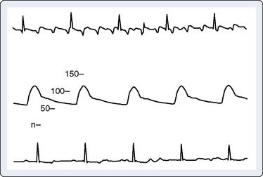
Figure 15-9 Baseline artifact simulates atrial flutter in a cannulated patient (top), with stable arterial pressure (middle) just before institution of full cardiopulmonary bypass, similar to that described by Kleinman et al.37 The “pseudoflutter waves” are corrected by application of the grounding cable (bottom).
(From London MJ, Kaplan JA: Advances in electrocardiographic monitoring. In Kaplan JA, et al (eds): Cardiac Anesthesia, 4th ed. Philadelphia: Saunders/Elsevier, 1999.)
ECG artifact often mimics arrhythmias, primarily atrial, because the baseline artifact may resemble flutter waves or atrial fibrillation. Kleinman et al37 (see earlier pump artifact) reported the commonly observed “atrial flutter” artifact (see Figure 15-9). Baseline artifact simulating flutter waves at 300 per minute occurred on an operating room monitor. The waves were observed to precisely track the pump head speed, disappearing when the pump was turned off. The artifact appears to have been caused by poor ECG electrode contact because the authors were able to produce it by undermining an ECG electrode with liquids. They pointed out that poor application of only one electrode can markedly impair the common-mode rejection capabilities of the ECG differential amplifier. This type of artifact also has been reported during noncardiac surgery.34 Other clinical devices associated with ECG interference, albeit rarely, include infusion pumps and blood warmers. Isolated power supply line isolation monitors have also been associated with 60-Hz interference. This can be diagnosed by removing the line isolation monitor fuses to see whether the artifact disappears.38

Frequency Response of Electrocardiographic Monitors: Monitoring and Diagnostic Modes
ECG signals must be amplified and filtered before display. Each must be amplified equally to reproduce the component frequencies accurately. The monitor must have a “flat amplitude response” over the wide range of frequencies present. Similarly, because the slight delay in a signal as it passes through a filter or amplifier may vary in duration with different frequencies, all frequencies must be delayed equally. This is termed linear phase response. If the response is nonlinear, various components may appear temporally distorted (called phase shift). Given the importance of the ECG in diagnosing myocardial ischemia, it is important to realize that “significant” ST-segment depression or elevation can occur solely as a result of improper signal filtering in 12-lead ECG machines and bedside or ambulatory ST-segment monitors.39–43 This artifact was a particular problem before the introduction of DSP. The AHA Committee on Electrocardiography Standardization has addressed specific frequency requirements for monitoring in this setting.6,26
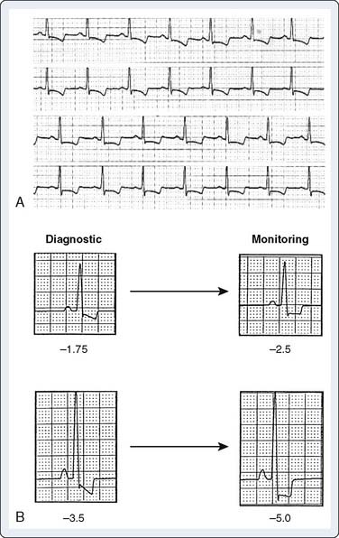
Nonlinear frequency response in the low-frequency range (0.5 Hz) can cause artifactual ST depression, whereas phase delay in this range can cause ST-segment elevation.6 The AHA recommends a bandwidth from 0.05 to 100 Hz (at 3 dB).30 Although a completely linear response is desirable, with analog filters, it is not generally possible. Because greater baseline noise is present when a 0.05-Hz cutoff is used, the 0.5-Hz cutoff often is used to display a more stable signal. This commonly is referred to as “monitoring mode,” and use of a 0.05-Hz low-frequency cutoff is known as “diagnostic mode.”44 The difference in ST-segment morphology at various low-frequency cutoffs is illustrated in Figure 15-10. Because most newer monitors use signal averaging techniques that effectively eliminate most artifact even in the diagnostic mode, the clinician can usually (and should) avoid using the monitoring mode, whenever possible.
High-frequency response is of less importance clinically because the ST segment and T wave reside in the low-frequency spectrum. However, at the commonly used high-frequency cutoff of 40 Hz, the amplitude of the R and S waves may diminish significantly, making it difficult to diagnose ventricular hypertrophy.40,45 Significant reduction in QRS amplitude may occur in the following circumstances: major decreases in LV function, obesity, pericardial and pleural effusions, anasarca, and infiltrative or restrictive cardiac diseases.46,47
Tsuda et al48 studied changes in R-wave amplitude in V5 throughout the intraoperative period in 35 patients undergoing CABG or valve replacement. Amplitude was reduced by 50% to 60% before institution of CPB. CABG patients had a slower recovery of R-wave amplitude. Marked reduction and failure of recovery of R-wave amplitudes occurred in patients who died perioperatively, a finding often observed clinically but not previously documented in the literature. Crescenzi et al49 have extended these observations by comparing R-wave amplitude in leads V4 and V5 in patients undergoing CABG with (n = 35) or without CPB (n = 35). A control group of patients undergoing mitral valve repair (n = 31) without CAD was included. A lack of change of amplitude in the R wave was found in the off-pump cases in contrast with reductions of R-wave amplitude in patients undergoing CABG or mitral valve surgery with CPB. Although biochemical markers of cardiac damage were significantly lower in the off-pump CABG group, no significant correlation was observed between alteration of R-wave amplitude and biochemical marker levels. It does not appear that fluid shifts or weight changes were considered in this analysis, factors that are more likely with the use of CPB. Larger sample sizes and more detailed analyses are required to better refine any potential clinically useful applications of QRS amplitude changes.
Electrocardiographic changes with myocardial ischemia

Detection of Myocardial Ischemia
The ST segment is the most important portion of the QRS complex for evaluating ischemia.50,51 It may come as a surprise that there are no gold standard criteria for the ECG diagnosis of myocardial ischemia. Many anesthesiologists, when evaluating an ECG for signs of ischemia, look for signs of repolarization or ST-segment abnormalities. There are also many other signs of myocardial ischemia that may be evidenced in the ECG. These include T-wave inversion, QRS and T-wave axis alterations, R- or U-wave changes, and the development of previously undocumented arrhythmias or ventricular ectopy.10 None of these, however, is as specific for ischemia as ST-segment depression or elevation.
Repolarization of the ventricle proceeds from the epicardium to the endocardium, opposite to the vector of depolarization. The ST segment reflects the midportion, or phase 2, of repolarization during which there is little change in electrical potential.52 It is usually isoelectric. Ischemia causes a loss of intracellular potassium, resulting in a current of injury. The electrophysiologic mechanism accounting for ST-segment shifts (elevation or depression) remains controversial. The two major theories are based on a loss of resting potential as current flows from the uninjured to the injured area (i.e., diastolic current) and on a true change in phase 2 potential as current flows from the injured to the uninjured area (i.e., systolic current; Figure 15-11). With subendocardial injury, the ST segment is depressed in the surface leads. With epicardial or transmural injury, the ST segment is elevated (Figure 15-12). When a lead is placed directly on the endocardium, opposite patterns are recorded.
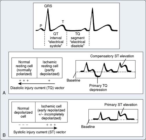
Figure 15-11 Pathophysiology of ischemic ST elevation.
(Reprinted from Mirvis DM, Goldberger AL: Electrocardiography. In Bonow RO, Mann DL, Zipes DP, Libby P (eds): Braunwald’s Heart Disease: A Textbook of Cardiovascular Medicine, 8th ed. Philadelphia: Saunders/Elsevier, p. 174, 2008.)
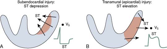
Figure 15-12 Current of injury patterns with acute ischemia.
(Reprinted from Mirvis DM, Goldberger AL: Electrocardiography. In Bonow RO, Mann DL, Zipes DP, Libby P (eds): Braunwald’s Heart Disease: A Textbook of Cardiovascular Medicine, 8th ed. Philadelphia: Saunders/Elsevier, p. 174, 2008.)
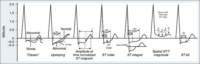
The classic criterion for ischemia is 0.1 mV (1 mm) of ST-segment depression measured 60 to 80 milliseconds after the J point (Figure 15-13).50,51 The slope of the segment must be horizontal or downsloping. Downsloping depression may be associated with a greater number of diseased vessels and a worse prognosis than horizontal depression. Slowly upsloping depression with a slope of 1 mV/sec or less is also used but is considered less sensitive and specific (and difficult to assess clinically). The magnitude of ST-segment depression is related directly to the height of the associated R wave. Given that R waves are highest in the lateral precordium and lowest in the inferior regions, some have proposed “normalizing” ST depression for this variable.53 However, this is controversial and not practical clinically. Nonspecific ST-segment depression can be related to drug use, particularly digoxin.54 Interpretation of ST-segment changes in patients with LV hypertrophy is particularly controversial given the tall R-wave baseline, J-point depression, and steep slope of the ST segment. Although a number of studies have excluded such patients, others (including those using other modalities or epidemiologic studies) observed that LV hypertrophy is a highly significant predictor of adverse cardiac outcome.55
The criteria for myocardial ischemia with ST-segment elevation (0.1 mV in two contiguous leads) are used in conjunction with clinical symptoms or elevation of biochemical markers to diagnose acute coronary syndromes. It usually results from transmural ischemia, but it may potentially represent a reciprocal change in a lead oriented opposite to the primary vector with subendocardial ischemia (as may be seen in the reverse situation).56,57 Perioperative ambulatory monitoring studies also have included more than 0.2 mV in any single lead as a criterion, but ST elevation rarely is reported in the setting of noncardiac surgery. It is commonly observed, however, during weaning from CPB in cardiac surgery and during CABG surgery (on- and off-pump) with interruption of coronary flow in a native or graft vessel. ST elevation in a Q-wave lead should not be analyzed for acute ischemia, although it may indicate the presence of a ventricular aneurysm.
Despite the clinical focus on the ST segment for monitoring, the earliest ECG change at the onset of transmural ischemia is the almost immediate onset of tall and peaked (i.e., hyperacute) T waves, a so-called primary change. This phase is often transient. A significant increase in R-wave amplitude may also occur at this time.58 T-wave inversions (symmetrical inversion) commonly accompany transmural ST-segment elevation changes, although most T-wave inversions or flattening observed perioperatively is nonspecific, resulting from transient alterations of repolarization because of changes in electrolytes, sympathetic tone, and other noncardiac factors.
Although repolarization changes (e.g., ST-T wave) are the focus of ischemia detection, computerized ECG analysis using signal averaging techniques has well-documented changes in depolarization with ischemia manifested by reduction in high-frequency components of the QRS complex (150 to 250 Hz). Such changes are not visible on the standard ECG, as they are in the range of only 10 to 20 mV, and are measured quantitatively using the root mean square (RMS) value (calculated by squaring the amplitude of each sample, determining the means of the squares, and then the square root of that mean value). Absolute changes in the RMS value greater than 0.6 mV or relative changes of more than 20% are considered clinically significant. This effect is likely due to slowing of conduction velocity in the ischemic region.59 One study documented higher sensitivity of this approach compared with 12-lead ST-segment analysis in the detection of acute coronary occlusion during percutaneous transluminal coronary angioplasty.60 The overall sensitivity was 88%, compared with 71% using ST-segment elevation criteria, or 79% by combining ST-segment elevation and depression. Its greatest value was in the detection of circumflex and right coronary artery occlusions.
Although this technology has been applied in several studies of patients undergoing cardiac surgery, all compared preoperative data with late (>1 week) postoperative data. Matsushita et al,61 however, described its perioperative use in 70 patients undergoing CABG or valve surgery, evaluating RMS values 1 to 2 hours after removal of the aortic crossclamp. Dividing patients into quartiles of RMS values, they observed that decreases in cardiac index correlated significantly with progressive reductions in RMS, use of inotropes, and longer cross-clamp times. At a threshold of 35% of preoperative values, a low cardiac output syndrome was more common. They hypothesized that the increase in intracellular calcium with ischemia is the common thread linking changes in conduction velocity with function. They recommended more common use of this technology because it is performed using an orthogonal lead set, which avoids the surgical field, is nearly real-time in nature, and extends the connection between ECG-derived parameters and cardiac function. Although intriguing, further studies from other groups clearly are required. It is unlikely this will be used commonly in the near future given the expense of replacing or upgrading existing equipment, but it remains a fertile topic for research.

Anatomic Localization of Ischemia with the Electrocardiogram
As noted earlier, ST-segment depression is a common manifestation of subendocardial ischemia. From a practical clinical standpoint, it has a single major strength and limitation. Its strength is that it is almost always present in one or more of the anterolateral precordial leads (V4 through V6).62 However, it fails to “localize” the offending coronary lesion and has little relation to underlying segmental asynergy.63,64
In contrast, ST elevation correlates well with segmental asynergy and localizes the offending lesion relatively well.63,65 Reciprocal ST-segment depression often is present in one or more of the other 12 leads. In patients with angiographically documented single-vessel disease, ST elevations (as well as Q waves or inverted T waves) in leads I, aVL, or V1 through V4 are closely correlated with disease of the left anterior descending artery, whereas similar findings in leads, II, III, and aVF indicate disease of the right coronary or left circumflex arteries (surprisingly, the latter two cannot be differentiated by ECG criteria).65 A multivariate analysis suggested that ST-segment elevation, abnormal Q waves, and inverted T waves in leads I and aVL (with normal V1 and V6) can be used to differentiate isolated first diagonal branch occlusion from the more ominous proximal left anterior descending artery occlusion.66
Berry et al64 demonstrated the insensitivity of surface leads relative to a unipolar intracoronary lead (the distal end of a guidewire across a coronary stenosis) for evaluating ischemia in certain regions of the heart during percutaneous transluminal coronary angioplasty. Occlusion of the left circumflex artery resulted in ST elevation in only 32% of patients on the surface ECG, primarily in the inferior leads (83%) or in V5 or V6 (33%).

Clinical Lead Systems for Detecting Ischemia
Early clinical reports of intraoperative monitoring using the V5 lead in high-risk patients were based on observations during exercise testing, in which bipolar configurations of V5 demonstrated high sensitivity for myocardial ischemia detection (up to 90%). Subsequent studies using 12-lead monitoring (torso mounted for stability during exercise) confirmed the sensitivity of the lateral precordial leads.67,68 Some studies, however, reported higher sensitivity for leads V4 or V6 compared with V5, followed by the inferior leads (in which most false-positive responses were reported).62,69–74
With the widespread growth of percutaneous coronary intervention for acute myocardial infarction and unstable angina in the 1990s, a number of investigators have reported on the use of continuous ECG monitoring (3 or 12 leads) in this setting. These observations have extended the classic teaching regarding localization of sites of coronary artery occlusion. Horacek and Wagner75 reviewed the complexities and controversies regarding vessel-specific ECG responses to acute myocardial ischemia in detail. In general, ST-segment elevation in leads V2 and V3 is most sensitive for occlusion of the left anterior descending coronary artery, and leads III and aVF are most sensitive for the right coronary artery. In contrast, circumflex occlusion results in variable responses, with primary elevation in the posterior precordial leads V7 through V9 (which are rarely monitored clinically), and reciprocal ST-segment depression in the standard precordial leads (V2 or V3).76,77 For transmural ischemia, sensitivity is highest in the anterior rather than the lateral precordial leads. An international multidisciplinary working group specifically recommended continuous monitoring of leads III, V3, and V5 for all acute coronary syndrome patients.78

Intraoperative Lead Systems
Detection of perioperative myocardial ischemia is an integral part of clinical monitoring and guides therapy (e.g., perioperative β-blockade). Many studies have demonstrated associations of perioperative ischemia with adverse cardiac outcomes in adults undergoing a variety of cardiac and noncardiac surgical procedures, particularly major vascular surgery.79–82 Perhaps the bigger challenge is interpreting minor ST-segment changes in the context of the overall risk profile of the patient to avoid costly diagnostic tests being performed inappropriately. Studies document that transient myocardial ischemia occurs in the absence of significant CAD in unexpected patients, such as parturients, particularly with significant hemodynamic stress or hemorrhage.83 Although the precise cause of such changes is uncertain, significant troponin release has been documented in these patients, confirming the suspicion that these ECG changes are true ischemic responses (probably related to subendocardial ischemia caused by global hypoperfusion).
How accurately the clinician places ECG leads on the patient’s torso is probably the single most important factor influencing clinical utility of the ECG. Placement of the limb leads almost anywhere on the torso at, or near the origin of, the arms allows accurate rendition of lead II because both electrodes are farther than 12 cm from the heart (a distance considered to be the electrical infinity value beyond which amplitude of the QRS complex is unchanged).84
The cardiac anesthesiologist encounters a variety of ECG changes consistent with or pathognomonic for myocardial ischemia or infarction at many phases of the perioperative period in patients undergoing cardiac surgery. In the majority of these patients (i.e., those with known CAD), the sensitivity and specificity of the major signs described later are high, and few false-positive or -negative changes are encountered. However, the abnormal physiology of CPB, including acute changes in temperature, electrolyte concentrations, catecholamine levels, and so on, can significantly influence sensitivity and specificity. In addition, patients undergoing valve replacement, even those without coronary artery lesions, can develop significant subendocardial and transmural ischemia (e.g., coronary artery embolus of valve calcification, vegetations, or air). Even neonates can experience development of myocardial ischemia85 (Figure 15-14).
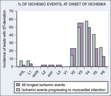
Detecting and recognizing the clinical significance of various ECG signs of ischemia or infarction can enhance patient care acutely, as in emergency treatment of coronary artery spasm or air embolus, or by alerting the surgeon that myocardial revascularization may have been inadequate. This may lead to re-exploration of a saphenous vein or internal mammary artery anastomosis, especially if the TEE data support the diagnosis of ischemia. The early reports of Kaplan87 and Dalton,86 recommending routine intraoperative monitoring of V5 in high-risk patients, cited exercise tolerance tests as the source of their recommendations (see Chapter 18). Subsequently, the recommended leads for intraoperative monitoring, based on several clinical studies, do not differ substantially from those used during exercise testing, although considerable controversy as to the optimal leads persists in both clinical settings. The coronary care unit’s use of continuous ECG monitoring has received increasing attention.88 A clinical study using continuous, computerized 12-lead ECG analysis in a mixed cohort (for vascular and other noncardiac procedures) by London et al89 reported that almost 90% of responses involved ST-segment depression alone (75% in V5 and 61% in V4). In approximately 70% of patients, significant changes were observed in multiple leads. The sensitivity of each of the 12 leads in that study is shown in Figure 15-15. When considered in combination (as occurs clinically), the use of leads V4 and V5 increased sensitivity to 90%, whereas sensitivity for the standard clinical combination of leads II and V5 was only 80%. Use of leads V2 through V5 and lead II captured all episodes (Table 15-3). A larger clinical study by Landesberg et al90 of patients undergoing vascular surgery, using a longer period of monitoring (up to 72 hours) with more specific criteria for ischemia (>10-minute duration of episode), extended these observations. They reported that V3 was most sensitive for ischemia (87%) followed by V4 (79%), whereas V5 alone was only 66% sensitive (Figure 15-16).90 In the subgroup of patients in whom prolonged ischemic episodes ultimately culminated in infarction, V4 was most sensitive (83%). In this study, all myocardial infarctions were non–Q-wave events detected by troponin elevation. Use of two precordial leads detected 97% to 100% of changes. Based on analysis of the resting isoelectric levels of each of the 12 leads (a unique component of this study), it was recommended that V4 was the best single choice for monitoring of a single precordial lead, because it was most likely to be isoelectric relative to the resting 12-lead preoperative ECG. In contrast, the baseline ST segment was more likely above isoelectric in V1 through V3 and below isoelectric in V5 and V6. Surprisingly, no episodes of ST elevation occurred in this study, as opposed to 12% in the earlier study of London et al,89 in which such changes were detected in inferior and anteroseptal precordial leads. Martinez et al91 evaluated a cohort of vascular surgical patients monitored in the intensive care unit for the first postoperative day with continuous 12-lead monitoring using a threshold of 20 minutes for an ischemic episode. Eleven percent of 149 patients met criteria, with ST depression in 71% and ST elevation alone in 18% (12% had both). Most changes were detected in V2 (53%) and V3 (65%). Using the standard two-lead system (II and V5), only 41% of episodes would have been detected. Although these studies clearly support the value of precordial monitoring in patients at risk for subendocardial ischemia, clinicians must be vigilant for the rare patient with acute Q-wave infarction (most commonly in the inferior leads). The studies previously cited have all been conducted in patients undergoing noncardiac surgery because it is not practical to conduct such studies in those with open chests or extensive surgical dressings in the precordial region. There is no reason, however, to assume that there would be any significant differences in the cardiac patient. Sudden episodes of acute transmural ischemia (associated with ST-segment elevation) are much more likely in this setting from acute ischemia/infarction (e.g., thrombotic occlusion) or surgery-induced reductions in coronary blood flow. The use of multiple precordial leads, although appealing, is not likely to become common clinical practice because of the limitations of existing monitors (and cables). Even if such equipment were available, it is likely that considerable resistance would occur from practitioners because of the extra effort associated with this approach. Perhaps, in the future, when lower cost wireless technologies are perfected, this approach may become a clinical reality.
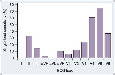
TABLE 15-3 Sensitivity for Different Electrocardiographic Lead Combinations
| Number of Leads | Combination | Sensitivity (%) |
|---|---|---|
| 1 lead | II V4 V5 |
33 61 75 |
| 2 leads | II/V5 II/V4 V4/V5 |
80 82 90 |
| 3 leads | V3/V4/V5 II/V4/V5 |
94 96 |
| 4 leads | II/V2-V5 | 100 |
Data from London MJ, Hollenberg M, Wong MG, et al: Intraoperative myocardial ischemia: Localization by continuous 12-lead electrocardiography. Anesthesiology 69:232, 1988.
Abnormalities in T-wave morphology are probably the most common perioperative ECG abnormality in the general surgical population. Breslow et al92 noted new T-wave abnormalities within 1 hour after surgery in 18% of an unselected surgical population of 394 patients (excluding cardiac and neurosurgery). About two thirds of the changes were limited to T wave flattening, and the remainder had new inversions. The incidence was no different between patients with known CAD and those without. Out of a battery of variables, the only one statistically associated with T-wave abnormalities was intra-abdominal surgery. Importantly, the ECG changes were not associated with any clinical morbidity. This study illustrates the known relation of T wave changes with a variety of autonomic stimuli, including changes in serum glucose, increased catecholamines, acute hyperventilation, and upper gastrointestinal disease. Similar analyses in patients undergoing cardiac surgery are not available, and the specificity of the response would be expected to be much lower.
Electrocardiographic changes with medications, electrolytes, and pacemakers
Use of inferior leads (II, III, aVF) allows superior discrimination of P-wave morphology, facilitating visual diagnosis of arrhythmias and conduction disorders. Although esophageal (and even intracardiac) leads allow the greatest sensitivity in detecting P waves, these rarely are used clinically. Nevertheless, they should be kept in mind for difficult diagnoses. With the increasing use of implantable defibrillators and automatic external defibrillators to treat ventricular fibrillation and ventricular tachycardia, there is considerable interest in the refinement of arrhythmia detection algorithms and their validation.93 As expected, the accuracy of the devices for detecting ventricular arrhythmias is high, but is much lower for detecting atrial arrhythmias. In the settings of critical care and ambulatory monitoring, a variety of artifacts are common causes of false-positive responses.93 Detection of pacemaker spikes may be complicated by very-low-amplitude signals related to bipolar pacing leads, amplitude varying with respiration, and total-body fluid accumulation.93,94 Most critical care and ambulatory monitors incorporate pacemaker spike enhancement for small high-frequency signals (typically 5 to 500 mV with 0.5- to 2-millisecond pulse duration) to facilitate recognition. However, this can lead to artifact if there is high-frequency noise within the lead system.
1 Munson E.S. Reports of scientific meetings. Anesthesiology. 1970;32:178-180.
2 American Society of Anesthesiologists. Standards for Basic Anesthetic Monitoring; 2005. 1-3
3 Hurst J.W. The renaissance of clinical electrocardiography. Heart Dis Stroke. 1993;2:290-295.
4 Kligfield P., Gettes L.S., Bailey J.J., et al. Recommendations for the standardization and interpretation of the electrocardiogram: Part I: The electrocardiogram and its technology: A scientific statement from the American Heart Association Electrocardiography and Arrhythmias Committee, Council on Clinical Cardiology; the American College of Cardiology Foundation; and the Heart Rhythm Society: Endorsed by the International Society for Computerized Electrocardiology. Circulation. 2007;115:1306-1324.
5 Weinfurt P.T. Electrocardiographic monitoring: An overview. J Clin Monit. 1990;6:132-138.
6 Tayler D.I., Vincent R. Artefactual ST segment abnormalities due to electrocardiograph design. Br Heart J. 1985;54:121-128.
7 Stern S. Angina pectoris without chest pain: Clinical implications of silent ischemia. Circulation. 2002;106:1906-1908.
8 Fleisher L.A., Beckman J.A., Brown K.A., et al. ACC/AHA 2007 Guidelines on Perioperative Cardiovascular Evaluation and Care for Noncardiac Surgery: Executive Summary: A Report of the American College of Cardiology/American Heart Association Task Force on Practice Guidelines. Circulation. 2007;116:1971-1996.
9 Cooper J.K. Electrocardiography 100 years ago. Origins, pioneers, and contributors. N Engl J Med. 1986;315:461-464.
10 Fisch C. Evolution of the clinical electrocardiogram. J Am Coll Cardiol. 1989;14:1127-1138.
11 Krikler D.M. The QRS complex. Ann N Y Acad Sci. 1990;601:24-30.
12 Rowlandson I. Computerized electrocardiography. A historical perspective. Ann N Y Acad Sci. 1990;601:343-352.
13 Fye W.B. A history of the origin, evolution, and impact of electrocardiography. Am J Cardiol. 1994;73:937-949.
14 Hurst J.W. Naming of the waves in the ECG, with a brief account of their genesis. Circulation. 1998;98:1937-1942.
15 Katz A.M. The Electrocardiogram, Physiology of the Heart. Philadelphia: Lippincott Williams & Wilkins, 2006;427-461.
16 Lynch C. Cellular electrophysiology of the heart. In: Lynch C., editor. Clinical Cardiac Electrophysiology. Philadelphia: JB Lippincott Company; 1994:1-52.
17 Rubart M., Zipes D.P. Genesis of cardiac arrhythmias: Electrophysiological considerations. In: Libby P., Bonow R.O., Mann D.L., Zipes D.P., editors. Brawnwald’s Heart Disease. Philadelphia: Saunders Elsevier; 2008:727-762.
18 Burger H.C. Heart-vector and leads. Br Heart J. 1946;8:157-161.
19 Burger H.C., Van Milaan J.B. Heart-vector and leads; geometrical representation. Br Heart J. 1948;10:229-233.
20 Carim H.M. Bioelectrodes. In: Webster J.G., editor. Encyclopedia of Medical Devices and Instrumentation. New York: John Wiley & Sons; 1988:195-224.
21 Plonsey R. Electrocardiography. In: Webster J.G., editor. Encyclopedia of Medical Devices and Instrumentation. New York: John Wiley & Sons; 1988:1017-1040.
22 Thakor N.V. Electrocardiographic monitors. In: Webster J.G., editor. Encyclopedia of Medical Devices and Instrumentation. New York: John Wiley & Sons; 1988:1002-1017.
23 Thakor N.V. Computers in electrocardiography. In: Webster J.G., editor. Encyclopedia of Medical Devices and Instrumentation. New York: John Wiley & Sons; 1988:1040-1061.
24 Kors J.A., van Bemmel J.H. Classification methods for computerized interpretation of the electrocardiogram. Methods Inf Med. 1990;29:330-336.
25 Sheffield L.T. Computer-aided electrocardiography. J Am Coll Cardiol. 1987;10:448-455.
26 Mirvis D.M., Berson A.S., Goldberger A.L., et al. Instrumentation and practice standards for electrocardiographic monitoring in special care units. A report for health professionals by a Task Force of the Council on Clinical Cardiology, American Heart Association. Circulation. 1989;79:464-471.
27 Watanabe K., Bhargava V., Froelicher V. Computer analysis of the exercise ECG: A review. Prog Cardiovasc Dis. 1980;22:423-446.
28 Bhargava V., Watanabe K., Froelicher V.F. Progress in computer analysis of the exercise electrocardiogram. Am J Cardiol. 1981;47:1143-1151.
29 Kossmann C.E. Unipolar electrocardiography of Wilson: A half century later. Am Heart J. 1985;110:901-904.
30 Pipberger H.V., ArzBaecher R.C., Golberger A.L. Recommendations for standardization of leads and of specifications for instruments in electrocardiography and vectorcardiography. Report of the Committee on Electrocardiography, American Heart Association. Circulation. 52, 1975.
31 Gardner R.M., Hollingsworth K.W. Optimizing the electrocardiogram and pressure monitoring. Crit Care Med. 1986;14:651-658.
32 de Pinto V. Filters for the reduction of baseline wander and muscle artifact in the ECG. J Electrocardiol. 1992;25(Suppl):40-48.
33 Levkov C., Mihov G., Ivanov R., et al. Removal of power-line interference from the ECG: A review of the subtraction procedure. Biomed Eng Online. 2005;4:50.
34 Lampert B.A., Sundstrom F.D. ECG artifact simulating supraventricular tachycardia during automated percutaneous lumbar discectomy. Anesth Analg. 1988;67:1096-1098.
35 Paulsen A.W., Pritchard D.G. ECG artifact produced by crystalloid administration through blood/fluid warming sets. Anesthesiology. 1988;69:803-804.
36 Khambatta H.J., Stone J.G., Wald A., Mongero L.B. Electrocardiographic artifacts during cardiopulmonary bypass. Anesth Analg. 1990;71:88-91.
37 Kleinman B., Shah K., Belusko R., Blakeman B. Electrocardiographic artifact caused by extracorporeal roller pump. J Clin Monit. 1990;6:258-259.
38 Marsh R. ECG artifact in the OR. Health Devices. 1991;20:140-141.
39 Berson A.S., Pipberger H.V. The low-frequency response of electrocardiographs, a frequent source of recording errors. Am Heart J. 1966;71:779-789.
40 Meyer J.L. Some instrument induced errors in the electrocardiogram. JAMA. 1967;201:351-356.
41 Bragg-Remschel D.A., Anderson C.M., Winkle R.A. Frequency response characteristics of ambulatory ECG monitoring systems and their implications for ST segment analysis. Am Heart J. 1982;103:20-31.
42 Bragg Remschel D. Silent myocardial ischemia. Problems with ST segment analysis in ambulatory ECG monitoring systems. In: Rutishauser W., Roskamm H., editors. Silent Myocardial Ischemia. Berlin: Springer Verlag; 1984:90-99.
43 Bailey J.J., Berson A.S., Garson A.Jr, et al. Recommendations for standardization and specifications in automated electrocardiography: Bandwidth and digital signal processing. A report for health professionals by an ad hoc writing group of the Committee on Electrocardiography and Cardiac Electrophysiology of the Council on Clinical Cardiology, American Heart Association. Circulation. 1990;81:730-739.
44 London M.J. Ischemia monitoring: ST segment analysis versus TEE. In: Kaplan J.A., editor. Cardiothoracic and Vascular Anesthesia Update. Philadelphia: WB Saunders Company; 1993:1-18.
45 Garson A.Jr. Clinically significant differences between the “old” analog and the “new” digital electrocardiograms. Am Heart J. 1987;114:194-197.
46 Madias J.E., Bazaz R., Agarwal H., et al. Anasarca-mediated attenuation of the amplitude of electrocardiogram complexes: A description of a heretofore unrecognized phenomenon. J Am Coll Cardiol. 2001;38:756-764.
47 Madias J.E. Recognizing the link between peripheral edema and voltage attenuation of QRS complexes: Implications for the critical care patient. Chest. 2003;124:2041-2044.
48 Tsuda H., Tobata H., Watanabe S., et al. QRS complex changes in the V5 ECG lead during cardiac surgery. J Cardiothorac Vasc Anesth. 1992;6:658-662.
49 Crescenzi G., Scandroglio A.M., Pappalardo F., et al. ECG changes after CABG: The role of the surgical technique. J Cardiothorac Vasc Anesth. 2004;18:38-42.
50 Fletcher G.F., Froelicher V.F., Hartley L.H., et al. Exercise standards. A statement for health professionals from the American Heart Association. Circulation. 1990;82:2286-2322.
51 Froelicher V.F. Interpretation of specific exercise test responses. In: Exercise and the Heart. Chicago: Year Book Medical Publishers; 1987:81-145.
52 Castellanos A., Interian A., Myerburg R. The resting electrocardiogram. In: Fuster V., Alexander R., O’Rourke R., editors. The Heart. ed 11. New York: McGraw-Hill; 2004:295-324.
53 Hollenberg M., Go M.Jr, Massie B.M., et al. Influence of R-wave amplitude on exercise-induced ST depression: Need for a “gain factor” correction when interpreting stress electrocardiograms. Am J Cardiol. 1985;56:13-17.
54 Goldberger A.L. Electrocardiogram in coronary artery disease: Limitations in sensitivity. In: Myocardial Infarction: Electrocardiographic Differential Diagnosis. St. Louis: CV Mosby; 1984:303-308.
55 Hollenberg M., Mangano D.T., Browner W.S., et al. Predictors of postoperative myocardial ischemia in patients undergoing noncardiac surgery. The Study of Perioperative Ischemia Research Group. JAMA. 1992;268:205-209.
56 Croft C.H., Woodward W., Nicod P., et al. Clinical implications of anterior S-T segment depression in patients with acute inferior myocardial infarction. Am J Cardiol. 1982;50:428-436.
57 Mirvis D.M. Physiologic bases for anterior ST segment depression in patients with acute inferior wall myocardial infarction. Am Heart J. 1988;116:1308-1322.
58 Brody D.A. A theoretical analysis of intracavitary blood mass influence on the heart-lead relationship. Circ Res. 1956;4:731-738.
59 Abboud S., Berenfeld O., Sadeh D. Simulation of high-resolution QRS complex using a ventricular model with a fractal conduction system. Effects of ischemia on high-frequency QRS potentials. Circ Res. 1991;68:1751-1760.
60 Pettersson J., Pahlm O., Carro E., et al. Changes in high-frequency QRS components are more sensitive than ST-segment deviation for detecting acute coronary artery occlusion. J Am Coll Cardiol. 2000;36:1827-1834.
61 Matsushita S., Sakakibara Y., Imazuru T., et al. High-frequency QRS potentials as a marker of myocardial dysfunction after cardiac surgery. Ann Thorac Surg. 2004;77:1293-1297.
62 Chaitman B.R., Hanson J.S. Comparative sensitivity and specificity of exercise electrocardiographic lead systems. Am J Cardiol. 1981;47:1335-1349.
63 Bar F.W., Brugada P., Dassen W.R., et al. Prognostic value of Q waves, R/S ratio, loss of R wave voltage, ST-T segment abnormalities, electrical axis, low voltage and notching: Correlation of electrocardiogram and left ventriculogram. J Am Coll Cardiol. 1984;4:17-27.
64 Berry C., Zalewski A., Kovach R., et al. Surface electrocardiogram in the detection of transmural myocardial ischemia during coronary artery occlusion. Am J Cardiol. 1989;63:21-26.
65 Fuchs R.M., Achuff S.C., Grunwald L., et al. Electrocardiographic localization of coronary artery narrowings: Studies during myocardial ischemia and infarction in patients with one-vessel disease. Circulation. 1982;66:1168-1176.
66 Iwasaki K., Kusachi S., Kita T., Taniguchi G. Prediction of isolated first diagonal branch occlusion by 12-lead electrocardiography: ST segment shift in leads I and aVL. J Am Coll Cardiol. 1994;23:1557-1561.
67 Blackburn H., Katigbak R. What electrocardiographic leads to take after exercise? Am Heart J. 1964;67:184-185.
68 Mason R.E., Likar I. A new system of multiple-lead exercise electrocardiography. Am Heart J. 1966;71:196-205.
69 Mason R.E., Likar I., Biern R.O., Ross R.S. Multiple-lead exercise electrocardiography. Experience in 107 normal subjects and 67 patients with angina pectoris, and comparison with coronary cinearteriography in 84 patients. Circulation. 1967;36:517-525.
70 Tubau J.F., Chaitman B.R., Bourassa M.G., Waters D.D. Detection of multivessel coronary disease after myocardial infarction using exercise stress testing and multiple ECG lead systems. Circulation. 1980;61:44-52.
71 Koppes G., McKiernan T., Bassan M., Froelicher V.F. Treadmill exercise testing. Part I. Curr Probl Cardiol. 1977;2:1-44.
72 Chaitman B.R., Bourassa M.G., Wagniart P., et al. Improved efficiency of treadmill exercise testing using a multiple lead ECG system and basic hemodynamic exercise response. Circulation. 1978;57:71-79.
73 Miller T.D., Desser K.B., Lawson M. How many electrocardiographic leads are required for exercise treadmill tests? J Electrocardiol. 1987;20:131-137.
74 Chaitman B.R. The changing role of the exercise electrocardiogram as a diagnostic and prognostic test for chronic ischemic heart disease. J Am Coll Cardiol. 1986;8:1195-1210.
75 Horacek B.M., Wagner G.S. Electrocardiographic ST-segment changes during acute myocardial ischemia. Card Electrophysiol Rev. 2002;6:196-203.
76 Carley S.D. Beyond the 12 lead: Review of the use of additional leads for the early electrocardiographic diagnosis of acute myocardial infarction. Emerg Med (Fremantle). 2003;15:143-154.
77 Zimetbaum P.J., Josephson M.E. Use of the electrocardiogram in acute myocardial infarction. N Engl J Med. 2003;348:933-940.
78 Drew B.J., Krucoff M.W. Multilead ST-segment monitoring in patients with acute coronary syndromes: A consensus statement for healthcare professionals. ST- Segment Monitoring Practice Guideline International Working Group. Am J Crit Care. 1999;8:372-386. quiz 387–388
79 Mangano D.T., Browner W.S., Hollenberg M., et al. Association of perioperative myocardial ischemia with cardiac morbidity and mortality in men undergoing noncardiac surgery. The Study of Perioperative Ischemia Research Group. N Engl J Med. 1990;323:1781-1788.
80 London M.J.T. The significance of perioperative ischemia in vascular surgery. In: Anesthesia Update. Cardiothoracic and Vascular Anesthesia. Philadelphia: WB Saunders Company; 1993:1-18.
81 Slogoff S., Keats A.S. Randomized trial of primary anesthetic agents on outcome of coronary artery bypass operations. Anesthesiology. 1989;70:179-188.
82 London M.J. Perioperative myocardial ischemia in patients undergoing myocardial revascularization. Curr Opin Anesthesiol. 1993;6:98.
83 Karpati P.C., Rossignol M., Pirot M., et al. High incidence of myocardial ischemia during postpartum hemorrhage. Anesthesiology. 2004;100:30-36. discussion 5A
84 Constant J. Learning electrocardiography. Boston: Little: Brown and Company, 1981.
85 Bell C., Rimar S., Barash P. Intraoperative ST-segment changes consistent with myocardial ischemia in the neonate: A report of three cases. Anesthesiology. 1989;71:601-604.
86 Dalton B. A precordial ECG lead for chest operations. Anesth Analg. 1976;55:740-741.
87 Kaplan J.A., King S.B.3rd. The precordial electrocardiographic lead (V5) in patients who have coronary-artery disease. Anesthesiology. 1976;45:570-574.
88 London M.J. Multilead precordial ST-segment monitoring: “The next generation?”. Anesthesiology. 2002;96:259-261.
89 London M.J., Hollenberg M., Wong M.G., et al. Intraoperative myocardial ischemia: Localization by continuous 12-lead electrocardiography. Anesthesiology. 1988;69:232-241.
90 Landesberg G., Mosseri M., Wolf Y., et al. Perioperative myocardial ischemia and infarction: Identification by continuous 12-lead electrocardiogram with online ST-segment monitoring. Anesthesiology. 2002;96:264-270.
91 Martinez E.A., Kim L.J., Faraday N., et al. Sensitivity of routine intensive care unit surveillance for detecting myocardial ischemia. Crit Care Med. 2003;31:2302-2308.
92 Breslow M.J., Miller C.F., Parker S.D., et al. Changes in T-wave morphology following anesthesia and surgery: A common recovery-room phenomenon. Anesthesiology. 1986;64:398-402.
93 Balaji S., Ellenby M., McNames J., Goldstein B. Update on intensive care ECG and cardiac event monitoring. Card Electrophysiol Rev. 2002;6:190-195.
94 Madias J.E. Decrease/disappearance of pacemaker stimulus “spikes” due to anasarca: Further proof that the mechanism of attenuation of ECG voltage with anasarca is extracardiac in origin. Ann Noninvasive Electrocardiol. 2004;9:243-251.
[/level-membership-for-anesthesiology-category][not-level-membership-for-anesthesiology-category]
15 Electrocardiographic Monitoring
As late as 1970, the electrocardiographic monitor was not considered an integral part of monitoring strategies in the perioperative period. As a matter of fact, luminaries in the specialty regarded the use of ECG monitoring as “questionable value because of possible iatrogenic problems.” Concern also was expressed that anesthesiologists’ attention would be diverted from the patient.1 Currently, monitoring the ECG is a fundamental standard of monitoring of the American Society of Anesthesiologists.2 Despite the introduction of more sophisticated cardiovascular monitors such as the pulmonary artery catheter and echocardiography, the electrocardiogram (ECG; coupled with blood pressure measurement) serves as the foundation for guiding cardiovascular therapeutic interventions in the majority of anesthetics.3 It is indispensable for diagnosing arrhythmias, acute coronary syndromes, electrolyte abnormalities, (particularly of serum potassium and calcium), and some forms of genetically mediated electrical or structural cardiac abnormalities (e.g., Brugada syndrome; Table 15-1).4
TABLE 15-1 Basic Clinical Information Available from Electrocardiography
| Anatomy or Morphology |
| Physiology |
One of the most important changes in electrocardiography that has occurred recently is the widespread use of computerized systems for recording ECGs. Bedside units are capable of recording diagnostic quality 12-lead ECGs that can be transmitted over a hospital network, for storage and retrieval. Most of the ECGs in the United States are recorded by digital, automated devices, equipped with software, which can measure ECG intervals and amplitudes and provide a virtually instantaneous interpretation. However, different automated systems may have different technical specifications that can result in significant differences in the measurement of amplitudes, intervals, and diagnostic statements.5,6 The diagnostic specificity and sensitivity of the ECG to diagnose a particular abnormality also are not consistent. For example, finite limits are defined by the relation between sensitivity and specificity (usually inversely related) for detecting obstructive coronary artery disease (CAD). During exercise testing, the 12-lead ECG has a mean sensitivity of only 68% and a specificity of 77%.7,8 The resting 12-lead ECG is even less sensitive and specific.8 More complex ECG modalities are likely to improve its utility in the future (high-frequency QRS signal averaging). In this chapter, the theory and the operating characteristics of ECG hardware used in the perioperative period are presented to facilitate proper use and interpretation of monitoring data.
Historical perspective
An extensive review of the history of electrocardiography is beyond the scope of this chapter. However, several excellent reviews were published in honor of the centennial of the first recording of the human ECG.9–14 Willem Einthoven is universally considered the father of electrocardiography (for which he won the 1924 Nobel Prize for Medicine/Physiology). Many of the basic clinical abnormalities in electrocardio-graphy were first described using the string galvanometer (e.g., bundle branch block, delta waves, ST-T changes with angina). It was used until the 1930s, when it was replaced by a system using vacuum tube amplifiers and a cathode ray oscilloscope. With advancements in electrical engineering technology, the devices became more compact, portable, and user friendly. In the 1950s, a portable direct-writing ECG cart was introduced. The first analog-to-digital (A/D) conversion systems for the ECG were introduced in the early 1960s, although their off-line use was impractical and restricted until the late 1970s. In the 1980s, microcomputer technology became widely available and is now standard for all diagnostic and monitoring systems. Further improvements in hardware and software design led to the development of automated ST-analysis algorithms and their use in routine clinical practice.
Basic electrophysiology and electrical anatomy of the heart
The ECG is the final result of a complex series of physiologic and technologic processes.15 Physiologically, the ECG reflects differences in transmembrane voltages in myocardial cells that occur during depolarization and repolarization within each cycle. Ionic currents are generated because of ionic fluxes across cell membranes in myocardial cells during depolarization and repolarization. The cardiac cells are con tiguous and electrically connected by ion channels (gap junctions), which allows the ion current to pass through the cells and spread depolarization.16 Thus, the membrane potential changes in the heart can be considered a single depolarization that propagates through the whole heart, assuming different forms along the way.16 The pattern and sequence of depolarization that occur in the heart are depicted in Figure 15-1. There are many different types and subtypes of ion channels that are involved in the synchronized generation of electrical activity in the heart. Of note are the sodium, potassium, calcium, and chloride channels.15–17 Detailed discussion of these channels is beyond the scope of this chapter.
At any point in time, the electrical activity of the heart is composed of differently directed electrical forces. However, these currents are synchronized by cardiac activation and recovery sequences to generate a cardiac electrical field in and around the heart that varies with time during the cardiac cycle. This cardiac electrical field passes through various internal structures such as lungs, blood, and skeletal muscles. The currents reaching the skin are then detected by the electrodes that are placed in specific locations on the body and uniquely configured to produce different ECG patterns or waveforms. Direction and strength of a lead vector depend on the geometry of the body and on the varying electric impedances of the tissues in the torso.18,19 As expected, placement of electrodes on the torso is distinct from direct placement on the heart because the localized signal strength that occurs with direct electrode contact is markedly attenuated and altered by torso inhomogeneities, which include thoracic tissue boundaries and variations in impedance. The standard 12-lead ECG records potential differences (represented as change of voltage over time) between prescribed sites on the body surface that vary during the cardiac cycle.4
The first deflection noted on the ECG is caused by atrial depolarization and is called the P wave. Although the depolarization of the sinoatrial node precedes the atrial depolarization (see Figure 15-1), the potential from these pacemaker cells are too small to be detected on the surface ECG. The width of the P wave reflects the time taken for the wave of depolarization to spread over both the right and left atria. In comparison with the ventricular action potential, the atrial action potential is narrower and has a less prominent plateau. The duration of atrial contraction is, thus, shorter, which permits another action potential to occur sooner and makes atria prone to a very high rate (atrial flutter). The repolarization atrial wave rarely is seen in a normal ECG because it is buried in the much larger QRS wave.
The ECG returns to its baseline between the end of atrial depolarization and the commencement of the QRS complex, which is the start of the QRS ventricular depolarization. This interval is called the PR interval. Though this period may seem electrically silent, it is a time of significant electrical activity. During this period, the wave of depolarization that started in the sinoatrial node is propagated through the AV node, the AV bundle, right and left bundle branches, and Purkinje fibers (see Figure 15-1).
The QRS wave is followed by a period when the ECG returns to the baseline and is called the ST segment. It is a time when the ventricle is completely depolarized and is represented by phase 2 of the action potential (see Figure 15-1). Even though the ventricles are depolarized, the ECG does not record any positive or negative waveforms because the whole ventricles are depolarized and there is no potential difference between sites. The ECG does not measure absolute levels of membrane potential but only records the potential differences.15 The same explanation also holds true for the T-P segment, which represents a time when the ventricles are fully repolarized; hence no significant potential difference is recorded on a surface ECG.
Sometimes small undulations can be seen after T waves but before P waves. These are called U waves and are thought to be generated by M cells, which are specialized midmyocardial cells with prolonged action potentials.15
Technical aspects of the electrocardiogram
Most clinicians assume that the ECG is a relatively simple technical device. However, an extensive amount of advanced electrical theory underlies both the recording and display of the ECG signal. Digital signal processing (DSP) is now used universally, and the average ECG unit incorporates several microprocessors. Anesthesiologists should familiarize themselves with the theory behind ECG acquisition to maximize rational clinical application and appreciate its clinical limitations. In this section, the basics of electrocardiography are presented, briefly considering the major components that are involved in the faithful rendition of the surface ECG, working from the skin and electrodes progressively to the final output on the screen. The reader is referred to a number of technical reviews for more detail.4,5,12,20–23
Processing of the ECG occurs in a series of steps as shown in Figure 15-2.4 These steps include (1) signal acquisition, including filtering; (2) data transformation, or rendition of data for further processing, including finding the complexes, classification of the complexes into “dominant” and “nondominant” (ectopic) types, and formation of an average or median complex for each lead; (3) waveform recognition, which is the process for identification of the onset and offset of the diagnostic waves; (4) feature extraction, which is the measurement of intervals and amplitudes; and (5) for the bedside 12-lead ECG machines, diagnostic classification.4 Diagnostic classification may be heuristic (i.e., deterministic, or based on experience-based rules) or statistical in approach.24
Figure 15-2 Schematic representation of the processes resulting in recording of the electrocardiogram.
Signal Acquisition and Power Spectrum of the Electrocardiogram
It is relevant to consider an electrocardiographic signal in terms of its amplitude (or voltage) and its frequency components (generally called its phase) to appreciate ECG signal acquisition. Voltage considerations differ depending on the signal source. Surface recording involves amplification of smaller voltages (on the order of 1 mV) than recording sites closer to the heart beneath the electrically resistant layers of the skin (e.g., endocardial, esophageal, and intratracheal leads). The “power spectrum” of the ECG (Figure 15-3) is derived by Fourier transformation, in which a periodic waveform is mathematically decomposed to its harmonic components (sine waves of various amplitudes and frequencies). The fundamental frequency for the QRS complex at the body surface is approximately 10 Hz, and most of the diagnostic information is contained below 100 Hz in adults. Spectra representing some of the major sources of artifact must be eliminated during the processing and amplification of the QRS complex.22 The frequency of each of these components can be equated to the slope of the component signal.6 The R wave with its steep slope is a high-frequency component (100 Hz), whereas P and T waves have lesser slopes and are lower in frequency (1 to 2 Hz). The ST segment has the lowest frequency, not much different from the “underlying” electrical (i.e., isoelectric) baseline of the ECG. Before the introduction of DSP, accurately displaying the ST segment presented significant technical problems, particularly in operating room and intensive care unit bedside monitoring units. Although the overall frequency spectrum of the QRS complex does not appear to exceed 40 Hz, many components of the QRS complex, particularly the R wave, can exceed 100 Hz. The American Heart Association (AHA) recommends a bandwidth of 0.05 to 100 Hz for monitoring and detection of myocardial ischemia.4 Very-high-frequency signals of particular clinical significance are pacemaker spikes. Their short duration and high amplitude present technical challenges for proper recognition and rejection to allow accurate determination of the heart rate. The frequencies of greatest importance for optimal ECG processing are presented in Table 15-2.5
TABLE 15-2 Range of Signal Frequencies Included in Different Phases of Processing in an Electrocardiographic Monitor
| Processing | Frequency Range |
|---|---|
| Display | 0.5 (or 0.05)–40 Hz |
| QRS detection | 5–30 Hz |
| Arrhythmia detection | 0.05–60 Hz |
| ST-segment monitoring | 0.05–60 Hz |
| Pacemaker detection | 1.5–5 kHz |
Digital Signal Processing of the Electrocardiogram
Computerized ECG processing has been adapted to all major clinical applications of the ECG. The earliest application of A/D signal processing occurred during exercise tolerance testing, when significant motion artifact and electromyographic noise make acquisition of a “clean” ECG signal difficult. Outside of the exercise treadmill laboratory, computer processing allows automated analysis of the diagnostic 12-lead ECG.25 The reader is referred elsewhere for more detailed discussions of this technology, and to the reports of the scientific council of the AHA on standardization and specifications for automated ECG and bedside monitors.4,25–28
Processing of the ECG signal by a digital electrocardiograph involves initial sampling of the signal from electrodes on the body surface. Nearly all current-generation ECG machines convert the analog ECG signal to digital form before further processing. The foundation of DSP is the A/D converter, which samples the incoming “continuous” analog signal (characterized by variable amplitude or voltage over time) at a very rapid rate, converting the sampled voltage into binary numbers, each of which has a precise time index or sequence. Greater sampling rates (≥ 10,000 to 15,000/sec), which are typically less than 0.5 millisecond in duration help detect pacemaker output reliably. Several technical recommendations regarding low-frequency filtering and high-frequency filtering recently have been published by the AHA.4
Formation of a Representative Single-Lead Complex
QRS waveform amplitudes and durations are subject to beat-to-beat variability and to respiratory variability between beats. Digital ECGs can adjust for respiratory variability and decrease beat-to-beat noise to improve the measurement precision in individual leads by forming a representative complex for each lead. Signal averaging is a critical component of this process. Noise is reduced using this technique proportionate by the square root of the number of beats averaged.4 Thus, a 10-fold reduction in noise is accomplished by averaging only 100 beats. Automated measurements are made from these representative templates, not from measurement of individual complexes. Average complex templates are formed from the average amplitude of each digital sampling point for selected complexes. Median complex templates are formed from the median amplitude at each digital sampling point. As a result, measurement accuracy is strongly dependent on the fidelity with which representative templates are formed. Because of the proprietary nature of this technology (the specific algorithms used are patented), the method used may vary by manufacturer. Consequently, the processed QRS complexes may vary in the “quality” of representation (i.e., if noise or aberrant beats are averaged into the complex, it will vary from the raw analog complex). The averaging process involves comparison of the voltages at a particular time point between the incoming complex and the template. Although the easiest method is to use the mean difference between voltages to update the “template,” the most accurate method is to use the median (because it is less affected by outliers, such as aberrant beats or other signals that have escaped QRS matching)4 (Figure 15-4).
A feature incorporated into most monitors is a visual trend line from which deviations in the position of the ST segment can be rapidly detected, which can aid online detection of ischemia. In addition, nearly all monitors display on-screen numerical values for the position of the ST segment used for ischemia detection (generally 60 to 80 milliseconds after the J point), although the specific fiducial point (based on heart rate) used usually can be adjusted by the clinician (Figure 15-5).
History and Description of the 12-Lead System
Where and how ECG electrodes are placed on the body are critical determinants of the morphology of the ECG signal. Lead systems have been developed based on theoretical considerations and references to anatomic landmarks that facilitate consistency between individuals (e.g., standard 12-lead system). Einthoven established electrocardiography using three extremities as references: the left arm, right arm, and left leg. He recorded the difference in potential between the left arm and right arm (lead I), between the left leg and right arm (lead II), and between the left leg and left arm (lead III) (Figure 15-6). Because the signals recorded were differences between two electrodes, these leads were called bipolar. The right leg served only as a reference electrode. Because Kirchoff’s loop equation states that the sum of the three voltage differential pairs must equal zero, the sum of leads I and III must equal lead II.21 The positive or negative polarity of each of the limbs was chosen by Einthoven to result in positive deflections of most of the waveforms and has no innate physiologic significance. He postulated that the three limbs defined an imaginary equilateral triangle with the heart at its center. Wilson refined and introduced the precordial leads into clinical practice. To implement these leads, he postulated a mechanism whereby the absolute level of electrical potential could be measured at the site of the exploring precordial electrode (the positive electrode). A negative pole with zero potential was formed by joining the three limb electrodes in a resistive network in which equally weighted signals cancel each other out. He called this the “central terminal,” and in a fashion similar to Einthoven’s vector concepts, he postulated it was located at the electrical center of the heart, representing the mean electrical potential of the body throughout the cardiac cycle. He described three additional limb leads (aVL, aVR, and aVF; Figure 15-7). These leads measured new vectors of activation, and in this way, the hexaxial reference system for determination of electrical axis was established. He subsequently introduced the six unipolar precordial V leads in 1935 (see Figure 15-6).29 Six electrodes are placed on the chest in the following locations: V1, fourth intercostal space at the right sternal border; V2, fourth intercostal space at the left sternal border; V3, midway between V2 and V4; V4, fifth intercostal space in the midclavicular line; V5, in the horizontal plane of V4 at the anterior axillary line, or if the anterior axillary line is ambiguous, midway between V4 and V6; and V6, in the horizontal plane of V4 at the midaxillary line4 (see Figure 15-6).
Clinical application of the unipolar limb leads was limited because of their significantly smaller amplitude relative to the bipolar limb leads from which they were derived. They were not clinically applied until Goldberger augmented their amplitude (by a factor of 1.5) by severing the connection between the central terminal and the lead extremity being studied (which he called “augmented limb leads”) in 1942. The limb leads, the precordial leads, and the augmented unipolar limb leads form what was accepted by the AHA as the conventional 12-lead ECG system.30 Einthoven’s law indicates that any one of the standard limb leads can be mathematically derived from the other two limb leads. Therefore, the “standard” 12-lead ECG actually contains eight independent pieces of information: two measured potential differences from which the four remaining limb leads can be calculated and the six independent precordial leads.4
[/not-level-membership-for-anesthesiology-category]
