[level-membership-for-internal-medicine-category]Chapter 24
Diagnostic Reasoning in Physical Diagnosis1
Medicine is a science of uncertainty and an art of probability. One of the chief reasons for this uncertainty is the increasing variability in the manifestations of any one disease.
Sir William Osler (1849–1919)
Art, Science, and Observation
This is one of the most important chapters of the book, because it considers the methods and concepts of evaluating the signs and symptoms involved in diagnostic reasoning. The previous chapters discuss the “science” of medicine by explaining the techniques for interviewing and performing the physical examination. The ability to make the “best” decision in the presence of uncertainty is the “art” of medicine. But there are rules and standards for the practice of this art, and these are the focus of this chapter.
The primary steps in this process involve the following:
Data collection is the product of the history and the physical examination. These can be augmented with laboratory and other test results such as blood chemistry profiles, complete blood cell counts, bacterial cultures, electrocardiograms, and chest radiographs. The history, which is the most important element of the database, accounts for more than 70% of the problem list. The physical examination findings contribute an additional 20% to 25% of the database; less than 10% of the database is related to laboratory and other test results.
Data processing is the clustering of data obtained from the history, physical examination, and laboratory and imaging studies. It is rare for patients to have a solitary symptom or sign of a disease. They more commonly complain of multiple symptoms, and the examiner may find several related signs during the physical examination. It is the job of the astute observer to fit as many of these clues together into a meaningful pathophysiologic relationship. This is data processing.
For example, suppose the interviewer obtains a history of dyspnea, cough, earache, and hemoptysis. Dyspnea, cough, and hemoptysis can be grouped together as symptoms suggestive of cardiopulmonary disease. Earache does not fit with the other three symptoms and may be indicative of another problem. For another patient who complains of epigastric burning relieved by eating and whose stool is found to contain blood, this symptom and this sign should be studied together. These data suggest an abnormality of the gastrointestinal tract, possibly a duodenal ulcer. Although patients usually have multiple symptoms or signs from a pathologic condition, they may not always manifest all the symptoms or signs of the disease being considered. For instance, the presence of polyuria and polydipsia in a patient with a family history of diabetes is adequate to raise the suspicion that a lateral rectus palsy may be related to diabetes, even if diabetes has not previously been diagnosed in this patient. In another patient, a 30-pound weight loss, anorexia, jaundice, and a left supraclavicular lymph node are suggestive of gastric carcinoma with liver metastasis to the porta hepatis. This illustrates the concept of data processing multiple symptoms into a single diagnosis. The process has sometimes been likened to the rule of Occam’s razor: The simplest theory is preferable—in this case, that all the symptoms can be explained by one diagnosis. Although it is a useful rule to keep in mind, it is not always applicable.
Problem list development results in a summary of the physical, mental, social, and personal conditions affecting the patient’s health. The problem list may contain an actual diagnosis or only a symptom or sign that cannot be clustered with other bits of data. The date on which each problem developed is noted. This list reflects the clinician’s level of understanding of the patient’s problems, which should be listed in order of importance. Table 24-1 is an example of a problem list.
Table 24–1
Example of a Problem List
| Problem | Date | Resolved |
| 1. Chest pain | 6/28/12 | |
| 2. Acute inferior myocardial infarction | 1/30/10 | 2/15/10 |
| 3. Colon cancer | 4/30/08 | 6/3/08 |
| 4. Diabetes mellitus | 2003 | |
| 5. Hypertension | 1997 | |
| 6. “Red urine” | 6/10/09 | 7/1/09 |
| 7. Distress over son’s drug abuse | 1/12 |
The presence of a symptom or sign related to a specific problem is a pertinent positive finding. For example, a history of gout and increased uric acid level are pertinent positive findings in a man suffering from excruciating back pain radiating to his testicle. This patient may be suffering from renal colic secondary to a uric acid kidney stone. The absence of a symptom or sign that, if present, would be suggestive of a diagnosis is a pertinent negative finding. A pertinent negative finding may be just as important as a pertinent positive finding; the fact that a key finding is not present may help rule out a certain diagnosis. For example, the absence of tachycardia in a woman with weight loss and a tremor makes the existence of hyperthyroidism less likely; the presence of tachycardia would strengthen the likelihood of hyperthyroidism.
An important consideration in any database is the patient’s demographic information: sex, age, ethnicity, and area of residence. A man with a bleeding disorder dating from birth is likely to have hemophilia. A 65-year-old person with exertional chest pain is probably suffering, statistically, from coronary artery disease. A 26-year-old African-American patient with multiple episodes of severe bone pain may be suffering from sickle cell anemia. A person living in the San Joaquin Valley who has pulmonary symptoms may have coccidioidomycosis. This information is often suggestive of a unifying diagnosis, but the absence of a “usual” finding should never totally exclude a diagnosis.
It has been said, “Common diseases are common.” This apparently simplistic statement has great merit because it underlines the fact that the observer should not assume an exotic diagnosis if a common one accurately explains the clinical state. (In contrast, if a common diagnosis cannot account for all the symptoms, the observer should look for another, less common diagnosis.) It is also true that “Uncommon signs of common diseases are more common than common signs of uncommon diseases.”
Finally, “A rare disease is not rare for the patient who has the disease.” If a patient’s symptoms and signs are suggestive of an uncommon condition, that patient may be the 1 in 10,000 with the disease. Nevertheless, statistics based on population groups provide a useful guide in approaching clinical decision-making for individual patients.
Diagnostic Reasoning from Signs and Symptoms
Unfortunately, decisions in medicine can rarely be made with 100% certainty. Probability weights the decision. Only if the cluster of symptoms, signs, and test results is unequivocal can the clinician be certain of a diagnosis. This does not occur often. How, then, can the clinician make the “best” decision—best in light of current knowledge and research?
Laboratory tests immediately come to mind. But signs and symptoms obtained from the patient’s history and physical examination perform the same function as laboratory tests, and the information and results obtained from signs, symptoms, and tests are evaluated in the same way and are subject to the same rules and standards of evidence for diagnostic reasoning. Also, signs and symptoms actually account for more (90%) of the developing problem list than do laboratory test results (<10%).
Sensitivity and Specificity
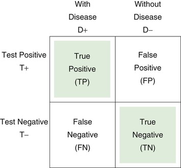
Throughout this text, signs and symptoms have been described according to their operating characteristics: sensitivity and specificity. These operating characteristics, which also apply to laboratory tests, indicate the usefulness of the sign, symptom, or test to the clinician in making a diagnosis. Sensitivity is equal to the true-positive rate, or the proportion of positive test results in individuals with a disease. Sensitivity, therefore, is based solely on patients with the disease. Specificity is equal to the true-negative (TN) rate, or the proportion of negative test results in individuals without a disease. Specificity, therefore, is based only on individuals without the disease. A false-positive (FP) finding refers to a positive test result in an individual without the disease or condition. Thus a sign, symptom, or test with 90% specificity can correctly identify 90 of 100 normal individuals; findings in the other 10 individuals are FP, and the FP rate is 10%. If a test result or observation is negative in a person with the disease, the result is termed false negative (FN).
The 2 × 2 table is useful for representing the relationship of a test, symptom, or sign to a disease. D+ indicates the presence of the disease; D− indicates the absence of the disease; T+ is a positive test result, or the presence of a symptom or sign; T− is the absence of a positive test result, or the absence of a symptom or sign. Each of the cells of the table represents a set of patients. Consider the following 2 × 2 table:
Sensitivity is defined as the number of true positive (TP) results divided by the number with disease (i.e., the total of the TP and the FN results):

Specificity is defined as the number of TN results divided by the number without disease (i.e., the total of FP results and TNs):

Substituting numbers:
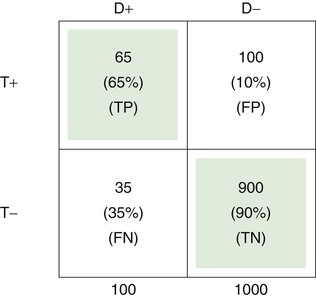
The upper left cell of the 2 × 2 table indicates that 65 of 100 patients with a certain disease (65%) had a certain positive test result or symptom or sign. Thus the test has a TP rate of .65, or a sensitivity of 65%.
The TN rate is .90, as indicated in the lower right cell; this means that 900 of 1000 individuals without the disease (90%) did not have a positive test result or symptom or sign. Therefore the specificity of the test is 90%.
The FP rate is .10, meaning that 100 of 1000 in the normal population (10%) had the finding for some reason, without having the disease in question. This is shown in the upper right cell.
Finally, the lower left cell indicates that the test result, symptom, or sign is absent in 35 of 100 patients with the disease. Thus the FN rate is 35%.
Note that the TP rate plus the FN rate equals 1; the FP rate plus the TN rate also equals 1. If the disease is aortic stenosis and the symptom is syncope, then according to the preceding table, 65% of patients with aortic stenosis have syncope, and 35% do not; 90% of individuals without aortic stenosis do not have syncope, and 10% do.
Likelihood Ratio
Because sensitivity and specificity are used to measure different properties, a symptom, sign, or test has both sensitivity and specificity values: high sensitivity and high specificity, low sensitivity and low specificity, high sensitivity and low specificity, or low sensitivity and high specificity. Sensitivity and specificity are often combined to form the likelihood ratio (LR), which provides a unitary measure of the operating characteristics of a sign, symptom, or test. The LR is defined as the ratio of the TP rate to the FP rate:

Thus the LR indicates the proportion of accurate to inaccurate positive test results. In the preceding example of syncope and aortic stenosis, where sensitivity = TP rate = .65, and 1 − specificity = FP rate = .10, the LR would be equal to .65/.10, or 6.5. In other words, a positive sign, symptom, or test result is 6.5 times more likely in patients with disease than in individuals without disease. In the example, the occurrence of syncope would be 6.5 times greater in patients with aortic stenosis than in individuals without it. Tests or signs with LRs greater than 10 are generally highly useful because they provide considerable confidence in diagnostic reasoning.
Ruling In and Ruling Out Disease
Sensitivity and specificity (and the LR) refer to properties of the symptom, sign, or test result that are invariant across different populations. This is true even though particular populations may differ with regard to the prevalence of the disease or condition in question. Sensitivity is based solely on patients with disease, and specificity is based solely on individuals without disease. Thus the relative sizes of the two groups—with disease and without disease—in the population of concern, which is the basis for the computation of prevalence, play no role in the computation of sensitivity and specificity. Sensitivity and specificity are simply the operating characteristics of the test and as such provide general information about the usefulness of the test for diagnostic reasoning with any population of patients. But in actual clinical practice, the clinician is concerned with the individual patient and whether that patient’s test results are predictive of disease. How certain can the clinician be that a patient has a disease if the test result is positive or if a symptom or sign is present? How certain can a clinician be that a person is healthy if a test result is negative or if a symptom or sign is absent? Typically, these questions are answered by computing the positive and negative predictive values, which are based on sensitivity and specificity but also take into account the prevalence of disease in the population of which the patient is a member.
First, however, consider two special cases of diagnostic reasoning in which clinical decisions can be based on only a knowledge of sensitivity and specificity. If the sensitivity of a given symptom, sign, or test is quite high, 90% or greater, and the patient has a negative result, the clinician can somewhat confidently rule out disease because so few patients with disease have a negative test result (<10%). Sackett (1992) devised the following acronym for this special case: Sensitive signs when Negative help rule out the disease (SnNout). In the absence of a highly sensitive sign, a person is most likely not to have the disease. The second special case occurs if the specificity of a given test, symptom, or sign is quite high, 90% or greater, and the patient has a positive result. The clinician can then somewhat confidently rule in disease because so few individuals without disease have a positive test result (<10%). Sackett’s acronym for this case is Specific signs when Positive help rule in the disease (SpPin). In the presence of a highly specific sign, a person is most likely to have the disease.
Positive and Negative Predictive Values
SnNout and SpPin are quite useful in those two special cases, but usually the clinician wants to predict the actual probability of disease for a patient with a positive result or the probability of no disease for an individual with a negative result. The former is estimated by the positive predictive value (PV+), which is equal to the number of TP findings divided by the total number of positive result findings in the population of which the patient is a member (the TP findings plus the FP findings):

The positive predictive value is the frequency of disease among patients with positive test results. Stated another way, it is the probability that a patient with a positive test result actually has the disease. The negative predictive value (PV−) is equal to the number of TN results divided by the total number of negative results in the patient’s population (the TN findings plus the FN findings):

The negative predictive value is the frequency of nondisease in individuals with negative test results. Stated another way, it is the probability of not having the disease if the test result is negative or if the symptom or sign is absent.

and the PV− is as follows:

Thus the predicted probability that a person with a positive result in fact has the disease is 39%. The predicted probability that a person with a negative result does not have the disease is 96%. In the hypothetical example, the probability that a patient with syncope actually has aortic stenosis is only 39%, whereas the probability that a person without syncope does not have aortic stenosis is 96%. The high PV− of 96% is consistent with the high test specificity of 90%.
Prevalence
Clearly, the sensitivity and specificity of a sign, symptom, or test are important factors in predicting the probability of disease, given the test results. So too is the prevalence of the disease in the population of which the patient is a member. The prevalence of disease refers to the proportion with disease in the population of interest. In a 2 × 2 table that represents the entire population (or a representative sample), prevalence is equal to the number with disease (TP + FN) divided by the total number in the population (TP + FP + FN + TN). Again, assuming that the preceding 2 × 2 table represents the entire population of concern, prevalence is calculated as follows:
Prevalence = (65 + 35)/(65 + 100 + 35 + 900) = 100/1100 = .09
Among this population, 9% have the disease in question.
Two intuitive examples illustrate the role of prevalence in predicting the probability of disease. Consider the value of the symptom of chest pain for predicting the probability of coronary artery disease. The first patient is a 65-year-old man with chest pain. The prevalence of coronary artery disease in the population of 65-year-old men is high. Therefore the presence of chest pain has a high positive predictive value for this patient, and it is probable that coronary artery disease exists in this patient. However, the absence of chest pain has a low negative predictive value, indicating that, because the prevalence is high, coronary artery disease may exist even in the absence of symptoms.
In contrast, consider the positive predictive value of chest pain in a 20-year-old woman. Among women in this age group, the prevalence of coronary artery disease is low, so the probability that this patient’s chest pain represents coronary artery disease is low. The presence of chest pain in a 20-year-old woman has a low positive predictive value. However, the absence of chest pain has a high negative predictive value, indicating that coronary artery disease is unlikely to be present.
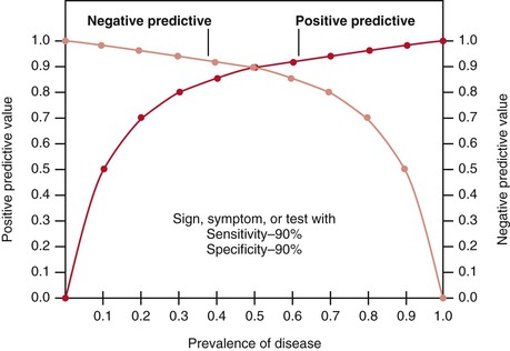
Figure 24-1 illustrates how changes in disease prevalence affect predictive values. The most significant increase in the positive predictive value of a sign, symptom, or test occurs when the disease is less common. At this end of the curve, small changes in prevalence produce great changes in the positive predictive value. Conversely, the most significant increase in the negative predictive value occurs when the disease is most prevalent. Slight decreases in the prevalence of common diseases produce significant increases in the negative predictive value. The higher the prevalence is, the higher the positive predictive value is and the lower the negative predictive value is.
Differences in prevalence rates may be related either to the clinical setting in which the patient is seen or to the specific demographic characteristics of the patient. For example, a clinician performing routine examinations in an outpatient clinic will find a prevalence of disease different from that found by a clinician working only with inpatients in a hospital specializing in that disease. The demographic characteristics of the patient refer to age, gender, and race, and these characteristics play a major role in the prevalence of many diseases. Both the clinical setting and the characteristics of the patient help determine the usefulness of the sign, symptom, or laboratory test because they affect both the positive and the negative predictive values of the finding.
Bayes’ Theorem
The formulas for PV+ and PV− are appropriate only if data in the 2 × 2 table are for the entire population or a representative sample of that population, in which case the prevalence of disease in the population is accurately reflected in the table. More typically, the sensitivity and specificity of the test, sign, or symptom are determined independently of the prevalence of disease, which must be ascertained by the clinician for the specific patient in question (e.g., prevalence of disease for the patient’s gender, age group, or ethnic group, or for inpatients versus outpatients). Thus the positive and negative predictive values are typically computed with Bayes’ theorem, which expresses PV+ and PV− as functions of sensitivity, specificity, and prevalence. To understand Bayes’ theorem, consider the tree diagram in Figure 24-2.
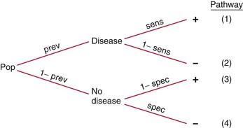
Figure 24–2 Tree diagram.
Consider again the example of syncope in patients with aortic stenosis, using the data in the 2 × 2 table. This time, do not assume that the data represent the entire population; assume that the data for the diseased and nondiseased groups were obtained separately, meaning that the prevalence of disease cannot be determined from the table, although sensitivity and specificity can be. Now assume that the prevalence of aortic stenosis is 80% in a given patient population. The sensitivity of syncope related to aortic stenosis remains 65% and the specificity 90%, as indicated in the table. Using Bayes’ theorem, calculate the PV+ and PV− as follows:


Thus a positive finding of syncope would increase the probability that the patient has aortic stenosis from 80% (the prevalence, or unconditional probability, of aortic stenosis in the general population) to 96% (the conditional probability of aortic stenosis in the presence of syncope). A negative finding for syncope would increase the probability of absence of stenosis from 20% (1 − prevalence in the general population) to 39% (the conditional probability of no stenosis in the absence of syncope). The absence of syncope in this patient has reduced the probability of aortic stenosis from 80% to 61% (100% − 39%).


Pursuing this example, now assume that the prevalence of aortic stenosis is only 20% in another patient population but that sensitivity and specificity remain at 65% and 90%, respectively. Bayes’ theorem now shows the PV+ and the PV− are as follows:


Notice that the PV+ has fallen from 96% (when prevalence was 80%) to 62% (with prevalence reduced to 20%). When the prevalence of a disease is quite low, the positive predictive value of a sign, symptom, or test is extremely low, even if the sensitivity and specificity are high. Also, notice that PV− has increased from 39% (when prevalence was 80%) to 91% (with prevalence reduced to 20%). Low prevalence of disease implies high negative predictive value. In general, with more disease (Prev ↑), more people with positive results will have the disease (PV+ ↑), and more people with negative results will have the disease (and fewer will not have the disease [PV− ↓]). In brief, as Prev ↑, PV+ ↑ but PV− ↓.
Nomogram
To simplify matters, a Bayes nomogram is given in Figure 24-3, which can be copied and used in the clinic or office. The nomogram provides the predictive values without requiring the calculations of Bayes’ theorem. To use the nomogram, first locate on the relevant axes the points that correspond to (1) the prevalence of disease for the patient’s population and (2) the LR for the sign, symptom, or test. Recall that the LR is the ratio of the TP rate (sensitivity) to the FP rate (1 − specificity). Next, place a straight edge on the nomogram to connect the points. The PV+ is given by the point at which the straight edge intersects the predictive value axis. For example, if prevalence = .80 and LR = .65/.10 = 6.50, the PV+ = .96, as computed earlier with Bayes’ theorem. To determine the PV−, use 1 − prevalence and TN rate divided by FN rate instead of prevalence and the LR.
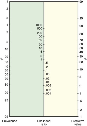
Figure 24–3 Nomogram for applying likelihood ratios.
Multiple Signs and Symptoms
Typically, diagnostic reasoning is based on multiple signs and symptoms and possibly on laboratory test results. These multiple findings must be combined to evaluate a diagnostic possibility. For example, consider the following clinical situation: A 21-year-old asymptomatic woman finds a thyroid nodule on self-examination, and she is referred to an endocrinologist for evaluation. The clinician describes the thyroid nodule as hard to palpation and fixed to the surrounding tissue. In this clinician’s practice, the prevalence of thyroid cancer is 3%. What is the chance that this nodule is cancerous?
To start, you can consider each finding separately. First, evaluate the predictive value of the presence of a palpable hard nodule. The sensitivity and specificity of this finding are 42% and 89%, respectively. With a prevalence of malignancy of 3%, Bayes’ theorem (or the nomogram) shows that the PV+ = 11% and the PV− = 98%. For the second finding, fixation of the nodule to the surrounding tissue, sensitivity is 31% and specificity is 94%. Again, with a prevalence equal to 3%, Bayes’ theorem (or the nomogram) shows that PV+ = 14% and PV− = 98%.
But what about the presence of both: a hard nodule that is fixed to the surrounding tissue? What about the presence of either a hard or a fixed nodule? Or the presence of neither? What are the predictive values of these combined findings? If it is assumed that the multiple signs, symptoms, and tests are independent (i.e., their findings are unrelated), the predictive values of these combined findings can be determined by extending the Bayesian tree diagram and adding a second finding, as shown in Figure 24-4.
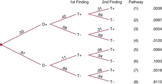
Figure 24–4 Extended tree diagram. D+, With disease; D−, without disease; T+, positive test result; T−, negative test result.


Notice that the positive predictive value for disease when both findings are positive (38%) is two to three times greater than the positive predictive value for a hard nodule only (11%) or for a fixed nodule only (14%).
In practice, multiple signs, symptoms, and test findings are typically not independent, because the presence of one finding increases the probability of the presence of another finding. Of course, the opposite is also possible, in that the second finding may be less likely in the presence of the first. Either way, the assumption of independence is violated, and the practice of calculating products of sensitivities in compound Bayesian trees (e.g., .42 × .31 in first pathway) does not produce accurate predictive values. Instead, the sensitivity and specificity for the actual compound finding must be known, such as the probability of the combined finding of a hard and fixed nodule. At present, this information is limited in the clinical research literature, but studies of compound findings with their sensitivities and specificities are increasing. It is hoped that this information will soon be available for clinical practice.
Decision Analysis
Diagnostic reasoning is only the first step in clinical decision-making. After reaching a decision about a diagnosis, the clinician must decide on a plan of treatment and management for the particular patient. These decisions must take into account the probability and utility (i.e., worth or value) of each possible outcome of the treatment or management plan, given the patient’s population (gender, age, ethnicity, inpatient or outpatient, and so forth). Similarly, the clinician may need to decide whether to order laboratory tests to confirm a diagnosis only suggested by the signs and symptoms elicited during the clinical examination. These test-ordering decisions must be based on the probability and utility of the possible outcomes of the test (possibly invasive and costly), and the patient’s population must again be taken into account. The purpose of this section is to extend the discussion of clinical decision-making to include making decisions about test ordering, treatment, and management.
Typically, a decision tree is used to represent the various alternatives, with probabilities assigned to the alternatives and utilities attached to the possible outcomes. Sackett and colleagues (1991) presented an excellent, detailed discussion of clinical decision-making. The following discussion relies on their test-ordering, decision-making example.
Their example involves “a 35 year old man with ‘heartburn’ for several years, no coronary risk factors, and a 6-week history of nonexertional, squeezing chest pain deep in his lower sternum and epigastrium, usually radiating straight through to his back and most likely to occur when he lies down after a heavy meal. He has a negative physical exam.”
The clinician in the example concludes that esophageal spasm is the best diagnosis and that significant coronary stenosis is very unlikely, perhaps 5% at most for this patient’s population. To address the latter possibility (serious, although unlikely), the clinician considers ordering exercise electrocardiography (E-ECG) just to be on the safe side, knowing that for greater than 70% stenosis, the sensitivity and specificity of E-ECG are 60% and 91%, respectively. According to this information and Bayes’ theorem (or the nomogram), PV+ = .26 and PV− = .98.
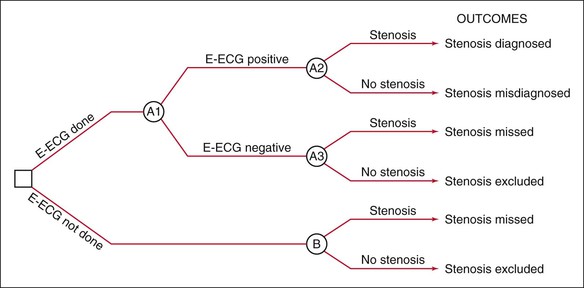
Construct Decision Tree
To decide whether to test with E-ECG, the clinician performs a decision analysis, first by constructing the decision tree in Figure 24-5, which depicts the decision-making situation. The clinician will decide whether to order E-ECG, as indicated on the left by the branching at the box-shaped “decision” node. If the clinician orders E-ECG, the results can be positive or negative, as shown by the next branching from the circular “chance” node; in either case, the patient can be found to have or not to have coronary stenosis, as shown by the branchings at the next two “chance” nodes. If the clinician decides not to order E-ECG, it is unknown whether the patient has the disease, as shown by the branching at the lower right “chance” node.
Assign Probabilities
Next, a probability is assigned to each branch in the tree, as shown in Figure 24-6. Ideally, probabilities should be based on strong clinical research studies. The proportions of patients with positive and negative E-ECG results are known to be 12% and 88%, respectively. Of those with positive results, 26% have stenosis and 74% do not. Notice that this first probability is the positive predictive value (PV+), which shows the proportion of individuals with a positive test result who do in fact have stenosis; the second proportion is 1 − PV+. Of those with negative results, the probabilities are 2% and 98%, respectively. The second probability here is the negative predictive value (PV−), and the first is 1 − PV−. In the general population not undergoing E-ECG, 5% have stenosis and 95% do not.
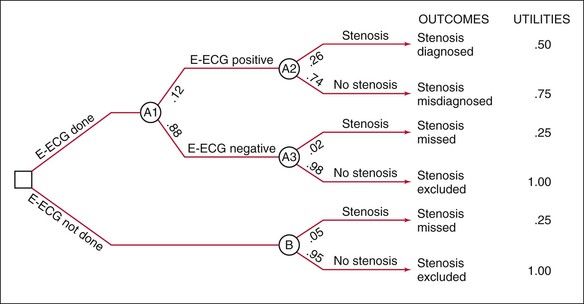
Attach Utilities
A utility is then attached to each of the possible outcomes, which are represented by the pathways through the tree. The utility refers to the worth, or value, of the outcome. Utilities may be objective, stated in monetary terms or expected years of life, or subjective, stated in relative terms of anticipated value to the patient or society. In the example, there are six outcomes (pathways through the tree), with a description or label for each outcome at the right of the pathway. A positive E-ECG result for a patient with stenosis, for example, is labeled “Stenosis diagnosed.” To the right of these labels are the utilities assigned by Sackett and colleagues (1991). These utilities are subjective, but they clearly show the relative worth of each of the outcomes: stenosis excluded (1, most valuable), stenosis misdiagnosed (.75), stenosis diagnosed (.50), and stenosis missed (.25, least valuable). The exact numerical value of each subjective utility is arbitrary, but the ordering of outcomes given by the utilities is not; that is, the same decision would be reached had the utilities been, say, 4, 3, 2, and 1, respectively. Of course, if the value of one outcome is much greater than that of a second, and the value of the second is similar to those of the third and fourth (e.g., 1, .50, .45, .40), the difference between the utilities for the first and second outcomes should be much greater than that between the second outcome and the third and fourth outcomes. This assignment of utilities could affect the decision reached.
Compute Expected Values
The expected value for each pathway through the tree is equal to the product of the probabilities and the utility for that outcome. For the first pathway, the expected value is given by .12 × .26 × .50 = .0156. The expected values for all six pathways, therefore, are .0156, .0666, .0044, .8622, .0125, and .9500. The expected value for each decision node is computed by summing the expected values for the outcomes originating from that node. For the decision to order E-ECG, the expected value is the sum of the expected values for the first four outcomes: .0156 + .0666 + .0044 + .8624 = .9490. For the decision not to order an E-ECG, the expected value is the sum of the last two outcomes: .0125 + .9500 = .9625.
Make a Decision
The expected value of the decision not to order E-ECG (.9625) is greater than that for ordering one (.9490). The decision analysis shows that the “best” decision for this patient is not to test. The decision would have been the same had the utilities been 4, 3, 2, 1 rather than 1, .75, .50, .25; the expected values for testing versus not testing would have been 3.796 and 3.850. Had the utilities been 1, .50, .45, and .40, the expected values would have been .928 and .970.
Clearly, the utilities, particularly subjective utilities, are the Achilles’ heel of decision analysis, although even objective utilities can be somewhat arbitrary. The expected values of the decision are affected by the utilities chosen for the analysis, and different utilities may lead to different decisions. Also, the probabilities assigned to the branches of the tree affect the outcome of the decision analysis, but the probabilities are typically less subjective than the utilities, being based on actual values such as sensitivities, specificities, and positive and negative predictive values obtained from the clinical research literature. Because the variability in the utilities and probabilities can affect the conclusion of the decision analysis, it has been suggested that the decision-maker systematically vary the utilities and probabilities within the reasonable range for the patient in question. This tests the vulnerability of the decision to reasonable variation in the utilities and probabilities. This is called a sensitivity analysis (although vulnerability analysis might be a better term, to avoid confusion with conventional test sensitivity). If the decision to test or not to test is consistent over these variations in utilities and probabilities, the clinician can be more confident in the decision. Otherwise, the decision is reduced to a toss-up between the alternatives.
In Sackett and colleagues’ example, the expected values for the decisions to test or not to test were quite close (.949 and .962), but they seem informative, at least intuitively, possibly because, surprisingly, they show a greater value for not testing. At the very least, the decision analysis shows that testing this patient is no better than not testing him. But what if the results were reversed, with the expected values for testing or not testing equal to .962 and .949, or with expected values for surgery or no surgery at .962 and .949? Close values such as these are not uncommon in decision analysis, and they illustrate the need to think clearly about the subjective meaning of the utility scale, which is given in terms of the nature of the outcomes to which the utilities are attached. For example, consider a four-point scale in which 4 represents stenosis excluded, 3 represents stenosis misdiagnosed, and so forth; the expected values for testing and not testing of 3.796 and 3.850, respectively, differ by only .054 of the unit distance between stenosis excluded (4) and stenosis misdiagnosed (3). The two decisions are closely valued. Nevertheless, in the absence of any other information, the “best” decision is not to test, which means simply that in the long run, with close-call decisions like this, there is a slight advantage to acting in accordance with the decision analysis.
The Rational Clinical Examination
In 1992, the Journal of the American Medical Association initiated a series of articles on the rational clinical examination. This series underscores the points made in this chapter: namely, that signs and symptoms provide critical information in diagnostic reasoning and that the operating characteristics (sensitivity and specificity) of the signs and symptoms must be considered in the reasoning process, as must the prevalence of the disease in question. In other words, the clinical examination can and should be more rational, based on empirical evidence of the predictive value of signs and symptoms used in diagnostic reasoning. A listing of the JAMA articles on the rational clinical examination since 1998 can be found in Appendix D, which is available in the online version of this textbook.
The rational clinical examination is part of a broader movement called evidence-based medicine, which “de-emphasizes intuition, unsystematic clinical experience, and pathophysiologic rationale as sufficient grounds for clinical decision-making and stresses the examination of evidence from clinical research.” The evidence-based approach to the practice of clinical medicine has its origins in clinical research generated within the relatively new field of clinical epidemiology. In the past, epidemiology was concerned with the causes of diseases, and hence the interest was in establishing that exposure to certain risk factors caused certain diseases. Thus classic epidemiology has been characterized as the study of the distribution of disease across time, place, and peoples. Clinical epidemiology has expanded this focus to encompass the study of the entire clinical process, including diagnosis, treatment, prognosis, prevention, evaluation of health care services, and risk-benefit analysis. Evidence from clinical research in these areas will probably be used to provide an empirical base for rational clinical practice, including diagnostic reasoning, as the “art” of clinical decision-making becomes more of a science.
The bibliography for this chapter is available at studentconsult.com.
Bibliography
Bowen JL. Educational strategies to promote clinical diagnostic reasoning. N Engl J Med. 2006;355:2217.
Bradley CP. Can we avoid bias? BMJ. 2005;330:784.
Brorsson B, Wall S. Assessment of medical technology: problems and methods. Swedish Medical Research Council: Stockholm; 1985.
Cutler P. Problem solving in clinical medicine: from data to diagnosis. ed 2. Williams & Wilkins: Baltimore; 1985.
Elstein AS, Schwarz A. Evidence base of clinical diagnosis: clinical problem solving and diagnostic decision making: selective review of the cognitive literature. BMJ. 2002;324:729.
Hunink M, et al. Decision making in health and medicine: integrating evidence and values. Cambridge University Press: New York; 2001.
Kassirer JP. Diagnostic reasoning. Ann Intern Med. 1989;110:893.
Lau AYS, Coiera EW. Do people experience cognitive biases while searching for information? J Am Med Inform Assoc. 2007;14:599.
Sackett DL. A primer on the precision and accuracy of the clinical examination. JAMA. 1992;267:2638.
Sackett DL, et al. Clinical epidemiology: a basic science for clinical medicine. ed 2. Little, Brown: Boston; 1991.
1 This chapter was written in collaboration with Jerry A. Colliver, PhD, and Ethan D. Fried, MD. Dr. Colliver is the former Director of Statistics and Research Consulting (1981–2007) and Professor of Medical Education at Southern Illinois University School of Medicine, Springfield, Illinois. Dr. Fried is Assistant Professor of Clinical Medicine at Columbia University College of Physicians and Surgeons, New York, New York.
[/level-membership-for-internal-medicine-category][not-level-membership-for-internal-medicine-category]Chapter 24
Diagnostic Reasoning in Physical Diagnosis1
Medicine is a science of uncertainty and an art of probability. One of the chief reasons for this uncertainty is the increasing variability in the manifestations of any one disease.
Sir William Osler (1849–1919)
Art, Science, and Observation
This is one of the most important chapters of the book, because it considers the methods and concepts of evaluating the signs and symptoms involved in diagnostic reasoning. The previous chapters discuss the “science” of medicine by explaining the techniques for interviewing and performing the physical examination. The ability to make the “best” decision in the presence of uncertainty is the “art” of medicine. But there are rules and standards for the practice of this art, and these are the focus of this chapter.
The primary steps in this process involve the following:
Data collection is the product of the history and the physical examination. These can be augmented with laboratory and other test results such as blood chemistry profiles, complete blood cell counts, bacterial cultures, electrocardiograms, and chest radiographs. The history, which is the most important element of the database, accounts for more than 70% of the problem list. The physical examination findings contribute an additional 20% to 25% of the database; less than 10% of the database is related to laboratory and other test results.
Data processing is the clustering of data obtained from the history, physical examination, and laboratory and imaging studies. It is rare for patients to have a solitary symptom or sign of a disease. They more commonly complain of multiple symptoms, and the examiner may find several related signs during the physical examination. It is the job of the astute observer to fit as many of these clues together into a meaningful pathophysiologic relationship. This is data processing.
For example, suppose the interviewer obtains a history of dyspnea, cough, earache, and hemoptysis. Dyspnea, cough, and hemoptysis can be grouped together as symptoms suggestive of cardiopulmonary disease. Earache does not fit with the other three symptoms and may be indicative of another problem. For another patient who complains of epigastric burning relieved by eating and whose stool is found to contain blood, this symptom and this sign should be studied together. These data suggest an abnormality of the gastrointestinal tract, possibly a duodenal ulcer. Although patients usually have multiple symptoms or signs from a pathologic condition, they may not always manifest all the symptoms or signs of the disease being considered. For instance, the presence of polyuria and polydipsia in a patient with a family history of diabetes is adequate to raise the suspicion that a lateral rectus palsy may be related to diabetes, even if diabetes has not previously been diagnosed in this patient. In another patient, a 30-pound weight loss, anorexia, jaundice, and a left supraclavicular lymph node are suggestive of gastric carcinoma with liver metastasis to the porta hepatis. This illustrates the concept of data processing multiple symptoms into a single diagnosis. The process has sometimes been likened to the rule of Occam’s razor: The simplest theory is preferable—in this case, that all the symptoms can be explained by one diagnosis. Although it is a useful rule to keep in mind, it is not always applicable.
Problem list development results in a summary of the physical, mental, social, and personal conditions affecting the patient’s health. The problem list may contain an actual diagnosis or only a symptom or sign that cannot be clustered with other bits of data. The date on which each problem developed is noted. This list reflects the clinician’s level of understanding of the patient’s problems, which should be listed in order of importance. Table 24-1 is an example of a problem list.
Table 24–1
Example of a Problem List
| Problem | Date | Resolved |
| 1. Chest pain | 6/28/12 | |
| 2. Acute inferior myocardial infarction | 1/30/10 | 2/15/10 |
| 3. Colon cancer | 4/30/08 | 6/3/08 |
| 4. Diabetes mellitus | 2003 | |
| 5. Hypertension | 1997 | |
| 6. “Red urine” | 6/10/09 | 7/1/09 |
| 7. Distress over son’s drug abuse | 1/12 |
The presence of a symptom or sign related to a specific problem is a pertinent positive finding. For example, a history of gout and increased uric acid level are pertinent positive findings in a man suffering from excruciating back pain radiating to his testicle. This patient may be suffering from renal colic secondary to a uric acid kidney stone. The absence of a symptom or sign that, if present, would be suggestive of a diagnosis is a pertinent negative finding. A pertinent negative finding may be just as important as a pertinent positive finding; the fact that a key finding is not present may help rule out a certain diagnosis. For example, the absence of tachycardia in a woman with weight loss and a tremor makes the existence of hyperthyroidism less likely; the presence of tachycardia would strengthen the likelihood of hyperthyroidism.
An important consideration in any database is the patient’s demographic information: sex, age, ethnicity, and area of residence. A man with a bleeding disorder dating from birth is likely to have hemophilia. A 65-year-old person with exertional chest pain is probably suffering, statistically, from coronary artery disease. A 26-year-old African-American patient with multiple episodes of severe bone pain may be suffering from sickle cell anemia. A person living in the San Joaquin Valley who has pulmonary symptoms may have coccidioidomycosis. This information is often suggestive of a unifying diagnosis, but the absence of a “usual” finding should never totally exclude a diagnosis.
It has been said, “Common diseases are common.” This apparently simplistic statement has great merit because it underlines the fact that the observer should not assume an exotic diagnosis if a common one accurately explains the clinical state. (In contrast, if a common diagnosis cannot account for all the symptoms, the observer should look for another, less common diagnosis.) It is also true that “Uncommon signs of common diseases are more common than common signs of uncommon diseases.”
Finally, “A rare disease is not rare for the patient who has the disease.” If a patient’s symptoms and signs are suggestive of an uncommon condition, that patient may be the 1 in 10,000 with the disease. Nevertheless, statistics based on population groups provide a useful guide in approaching clinical decision-making for individual patients.
Diagnostic Reasoning from Signs and Symptoms
Unfortunately, decisions in medicine can rarely be made with 100% certainty. Probability weights the decision. Only if the cluster of symptoms, signs, and test results is unequivocal can the clinician be certain of a diagnosis. This does not occur often. How, then, can the clinician make the “best” decision—best in light of current knowledge and research?
Laboratory tests immediately come to mind. But signs and symptoms obtained from the patient’s history and physical examination perform the same function as laboratory tests, and the information and results obtained from signs, symptoms, and tests are evaluated in the same way and are subject to the same rules and standards of evidence for diagnostic reasoning. Also, signs and symptoms actually account for more (90%) of the developing problem list than do laboratory test results (<10%).
Sensitivity and Specificity
Throughout this text, signs and symptoms have been described according to their operating characteristics: sensitivity and specificity. These operating characteristics, which also apply to laboratory tests, indicate the usefulness of the sign, symptom, or test to the clinician in making a diagnosis. Sensitivity is equal to the true-positive rate, or the proportion of positive test results in individuals with a disease. Sensitivity, therefore, is based solely on patients with the disease. Specificity is equal to the true-negative (TN) rate, or the proportion of negative test results in individuals without a disease. Specificity, therefore, is based only on individuals without the disease. A false-positive (FP) finding refers to a positive test result in an individual without the disease or condition. Thus a sign, symptom, or test with 90% specificity can correctly identify 90 of 100 normal individuals; findings in the other 10 individuals are FP, and the FP rate is 10%. If a test result or observation is negative in a person with the disease, the result is termed false negative (FN).
The 2 × 2 table is useful for representing the relationship of a test, symptom, or sign to a disease. D+ indicates the presence of the disease; D− indicates the absence of the disease; T+ is a positive test result, or the presence of a symptom or sign; T− is the absence of a positive test result, or the absence of a symptom or sign. Each of the cells of the table represents a set of patients. Consider the following 2 × 2 table:
Sensitivity is defined as the number of true positive (TP) results divided by the number with disease (i.e., the total of the TP and the FN results):
Specificity is defined as the number of TN results divided by the number without disease (i.e., the total of FP results and TNs):
Substituting numbers:
The upper left cell of the 2 × 2 table indicates that 65 of 100 patients with a certain disease (65%) had a certain positive test result or symptom or sign. Thus the test has a TP rate of .65, or a sensitivity of 65%.
The TN rate is .90, as indicated in the lower right cell; this means that 900 of 1000 individuals without the disease (90%) did not have a positive test result or symptom or sign. Therefore the specificity of the test is 90%.
The FP rate is .10, meaning that 100 of 1000 in the normal population (10%) had the finding for some reason, without having the disease in question. This is shown in the upper right cell.
Finally, the lower left cell indicates that the test result, symptom, or sign is absent in 35 of 100 patients with the disease. Thus the FN rate is 35%.
Note that the TP rate plus the FN rate equals 1; the FP rate plus the TN rate also equals 1. If the disease is aortic stenosis and the symptom is syncope, then according to the preceding table, 65% of patients with aortic stenosis have syncope, and 35% do not; 90% of individuals without aortic stenosis do not have syncope, and 10% do.
Likelihood Ratio
Because sensitivity and specificity are used to measure different properties, a symptom, sign, or test has both sensitivity and specificity values: high sensitivity and high specificity, low sensitivity and low specificity, high sensitivity and low specificity, or low sensitivity and high specificity. Sensitivity and specificity are often combined to form the likelihood ratio (LR), which provides a unitary measure of the operating characteristics of a sign, symptom, or test. The LR is defined as the ratio of the TP rate to the FP rate:
Thus the LR indicates the proportion of accurate to inaccurate positive test results. In the preceding example of syncope and aortic stenosis, where sensitivity = TP rate = .65, and 1 − specificity = FP rate = .10, the LR would be equal to .65/.10, or 6.5. In other words, a positive sign, symptom, or test result is 6.5 times more likely in patients with disease than in individuals without disease. In the example, the occurrence of syncope would be 6.5 times greater in patients with aortic stenosis than in individuals without it. Tests or signs with LRs greater than 10 are generally highly useful because they provide considerable confidence in diagnostic reasoning.
Ruling In and Ruling Out Disease
Sensitivity and specificity (and the LR) refer to properties of the symptom, sign, or test result that are invariant across different populations. This is true even though particular populations may differ with regard to the prevalence of the disease or condition in question. Sensitivity is based solely on patients with disease, and specificity is based solely on individuals without disease. Thus the relative sizes of the two groups—with disease and without disease—in the population of concern, which is the basis for the computation of prevalence, play no role in the computation of sensitivity and specificity. Sensitivity and specificity are simply the operating characteristics of the test and as such provide general information about the usefulness of the test for diagnostic reasoning with any population of patients. But in actual clinical practice, the clinician is concerned with the individual patient and whether that patient’s test results are predictive of disease. How certain can the clinician be that a patient has a disease if the test result is positive or if a symptom or sign is present? How certain can a clinician be that a person is healthy if a test result is negative or if a symptom or sign is absent? Typically, these questions are answered by computing the positive and negative predictive values, which are based on sensitivity and specificity but also take into account the prevalence of disease in the population of which the patient is a member.
[/not-level-membership-for-internal-medicine-category]
