A schematic of the general approach to modeling multi-scale cardiac electromechanical function at the level of the organ is shown in Figure 36-1, A. The general approach consists of two coupled problems, simulating the electrical and mechanical functions of the heart. A flowchart of the simulation process with connections within the model representation of each function as well as inter-relations between the two parts of the electromechanical model is presented in Figure 36-1, B.

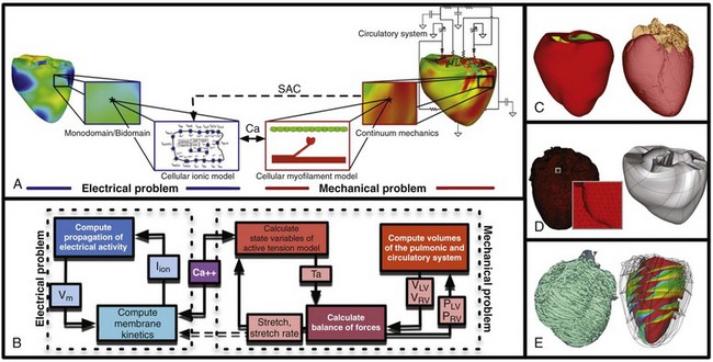
Figure 36-1 A, Schematic of the general approach to modeling cardiac electromechanical function. B, Flowchart of the simulation process. C, Geometric models of the heart (rabbit and canine). D, Computational meshes of the canine heart for electrical and mechanical problems. E, Fiber and sheet orientations obtained from diffusion tensor (DT)-magnetic resonance imaging (MRI) of the canine heart. (Images modified with permission from Vadakkumpadan F, Arevalo H, Prassl AJ, et al: Image-based models of cardiac structure in health and disease. Wiley Interdiscip Rev Syst Biol Med 2:489–506, 2010; Gurev V, Lee T, Constantino J, et al: Models of cardiac electromechanics based on individual hearts imaging data: Image-based electromechanical models of the heart. Biomech Model Mechanobiol 10:295–306, 2011.)

The electrical problem of the model simulates the propagation of a wave of transmembrane potential by solving the monodomain reaction-diffusion partial differential equation (PDE; or a system of coupled PDEs if the extracellular current flow is explicitly accounted for, i.e., the bidomain problem) over the volume of the heart.¹ The reaction-diffusion PDE describes current flow through myocytes that are electrically connected via low-resistance gap junctions. Cardiac tissue has orthotopic passive electrical conductivities that arise from the cellular organization of the heart into fibers and laminar sheets. Global conductivity values are obtained by combining fiber and sheet organization with myocyte-specific local conductivity values. Current flow in the tissue is driven by the active processes of ionic exchanges across myocyte membranes. These processes are represented by the cellular ionic model (see Figure 36-1, A, B), where current flow through ion channels, pumps, and exchangers and subcellular calcium cycling are governed by a set of ordinary differential (ODE) and algebraic equations; ionic models of different complexity are currently in use.² Simultaneous solution of the PDE(s) with the set of ionic model equations represents simulation of electrical wave propagation in the heart.

The intracellular calcium released during electrical activation couples the electrical and mechanical components of the model by providing a bi-directional link between the cellular ionic and myofilament models (see Figure 36-1, A, B). The cellular myofilament model consists of another set of ODEs that represent the biophysical processes of calcium binding to troponin and cross-bridge cycling, as well as the mechanisms of cooperativity. Compared with the evolution of cellular ionic models, the development of myofilament models has been slower and more difficult, as no clear consensus has been reached regarding the mathematical approach to model myofilament dynamics. An up-to-date review of cellular myofilament models can be found in a recent publication.³

The contraction of the heart arises from the active tension generated by the myofilaments within the cardiac cell. In the mechanics part of the model, deformation of the organ is described by the equations of continuum mechanics,⁴ with the passive properties of the myocardium described by a constitutive law. The most comprehensive formulation of cardiac tissue constitutive relation can be found in a recent article by Holzapfel and Ogden.⁵ Simultaneous solution of the myofilament model equations and of those representing passive cardiac mechanics over the volume of the heart (see Figure 36-1, A, B) constitutes simulation of cardiac contraction. Finally, to simulate the cardiac cycle and the corresponding pressure-volume loops, conditions on chamber volume and pressure are imposed, arising typically from lumped-parameter models of the systemic and pulmonic circulatory systems (see Figure 36-1, A, B).

In addition to the bi-directional relationship between electrical and mechanical components, provided by intracellular calcium cycling, a key feedback mechanism in the electromechanical model (acting within the mechanics component) is the length and velocity dependence of tension (see Figure 36-1, B): The stretch and stretch rate, as determined by the deformation of the heart, affect tension development in the cell. Mechanical deformation could further affect the electrical activity of the heart via the opening of stretch-activated channels (see Figure 36-1, A, B). To simulate this feedback mechanism, the stretch and stretch rate calculated from the mechanics component serve as an input into the electrical component: They determine the conductance of stretch-activated channels, the latter represented within the cellular ionic model.

Solutions to organ-level electromechanical problems entail the use of organ-level geometries, which could be idealized (such as cylindrical and elliptical shapes to represent the ventricles) or anatomically accurate, the latter representing ventricular averaged geometries obtained from histologic sectioning 6–8 or the geometry and structure of individual hearts,^9–11 as obtained from magnetic resonance imaging (MRI).¹² Figure 36-1, C presents some of the ventricular geometries used in electromechanical modeling: The University of California San Diego (UCSD) rabbit ventricular geometry⁶ is an example of averaged geometry obtained through histologic sectioning, while another image exemplifies an MRI-based individual heart geometry.⁹ An example of an MRI-based atrial geometry only can be found in a recent publication.¹³

The aforesaid description of electromechanical modeling refers to models of strong coupling, where the electrical and mechanical problems are solved simultaneously.¹⁴ In cases that do not necessitate strong coupling, as for instance during examination of how the mechanical activation of the heart follows the electrical activation, weakly coupled schemes are employed. In a weakly coupled model, the electrical activation times (calculated from the electrical problem) are inputted into the mechanical part as the instances when the myofilament model is activated. In a more sophisticated approach, the ionic and cardiac myofilament models can be coupled within the mechanics component, with the electrical activation times determining the instant at which this combined ionic-myofilament model is activated¹⁰; in this case, cooperativity mechanisms, such as calcium binding to troponin C, are represented in the model.

The governing equations describing cardiac electromechanical behavior are solved on a spatially discretized version of the heart volume (i.e., on the computational mesh). The electrical and mechanical parts of the model have different requirements regarding the degree of discretization (i.e., element size) and the element type; thus the two parts of the model require two different computational meshes. The electrical mesh requirements are based on spatiotemporal characteristics of wave propagation; a spatial resolution of about 250 to 300 micrometers is appropriate for electrophysiological finite element models. A novel approach was recently published for electrical mesh generation directly from segmented MRI ¹⁵ (Figure 36-1, D). The mechanical mesh, on the other hand, typically consists of hexahedral elements with a Hermite basis. This choice of finite elements increases the degree of strain continuity and is appropriate for maintaining incompressibility constraints. The mechanical mesh of the heart (see Figure 36-1, D) can also be generated directly from segmented MRI.^10,16

Fiber and laminar sheet organization underlies the orthotropic electrical conductivities of the tissue and its mechanical properties. In the electrical mesh, local fiber and sheet directions are typically mapped at the centroids of the finite elements, and in the mechanics mesh, fiber and sheet orientations and their derivatives are defined at mesh nodes and then are interpolated over the elements. This is typically done using histologic sectioning information ⁶ or diffusion tensor (DT) MRI data.^9,10 Use of DT-MRI data is based on the fact that the primary, secondary, and tertiary eigenvectors of the water DTs are aligned with fiber direction, with the direction transverse to the fiber direction and in the plane of the laminar sheet, and with that normal to the laminar sheet, respectively.¹² Figure 36-1, E presents fiber and sheet orientation, as reconstructed from DT-MRI of the canine heart. In cases where neither histologic nor DT-MRI information is available, rule-based approaches¹⁷ or image transformation algorithms¹⁸ have been used to assign fiber and sheet orientation consistent with measurements.

Simulations of heart electromechanical function are typically executed on parallel high-performance computing hardware. Reviews of numeric approaches to simulating the electromechanical activity of the heart can be found 1,10,19,20; these articles also address the challenges involved in developing multi-scale models at the organ level.

Approaches to Experimental Validation of Electromechanical Models

Validating the ventricular (or atrial) model of cardiac electromechanics with experimental data is a pivotal component of model development. It constrains the model parameter space and enhances the physiological relevance of the model. To validate the electrical component of the model, simulation results are often compared with electrical activation maps obtained from epicardial sock or plunge electrodes, from optical mapping, or from electrocardiograms (ECGs) and body surface potential maps. The mechanical component is validated with local strain measurements calculated from MRI or ultrasound images, or with hemodynamical metrics such as left ventricular (LV) pressure and volume, ejection fraction, or maximal rate of pressure change.

A study by Provost et al ²¹ provides a unique example of electromechanical (rather than separate electrical or mechanical) heart model validation. It is based on the use of electromechanical wave imaging (EWI),²² a novel noninvasive ultrasound-based imaging technique capable of mapping the propagation of the electromechanical wave along echocardiographic planes; this is achieved by mapping the interframe axial strains. In the Provost et al study,²¹ data from EWI were used to validate the MRI-based electromechanical model of the normal canine ventricles for different pacing protocols. Figure 36-2, A, B presents experimental and simulated EWI maps for pacing from the LV base; the corresponding isochronal maps of electromechanical activation are shown in Figure 36-2, C. In both experiments and simulations, the EW emerged from the basal region of the lateral wall and propagated toward the apex, the septum, and the right ventricular (RV) wall. Representative curves of the interframe strains over time in the lateral and septal wall are shown in Figure 36-2, D. This study provides an illustrative example of how emerging experimental techniques like EWI could be used for validation of cardiac electromechanical models.

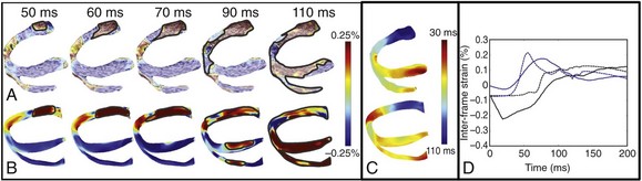
Figure 36-2 Validation of the electromechanical model of the canine heart with electromechanical wave imaging. Experimental (top) and simulated (bottom) interframe strain distribution associated with an electromechanical wave (A) and the corresponding isochronal maps of electromechanical activation (B) for LV base pacing. C, Experimental and simulated interframe strain traces at the septum (black) and the lateral wall (blue). (Images modified with permission from Provost J, Gurev V, Trayanova N, et al: Mapping of cardiac electrical activation with electromechanical wave imaging: An in silico-in vivo reciprocity study. Heart Rhythm 8:752–759, 2011.)

Applications of Electromechanical Modeling

Electromechanical Interactions in the Heart

Understanding the mechanical consequences of an altered cardiac activation sequence is of great importance because dyssynchronous electrical activation can cause abnormalities in perfusion and pump function. Early computational studies of electromechanics employed truncated ellipsoids as LV representations in an attempt to provide insight into the relationship between the spatial pattern of electrical activation and the resultant contraction.²³ The study by Usyk and McCulloch²⁴ was the first to examine the distribution of the time interval between myocyte depolarization and onset of myofiber shortening, termed the electromechanical delay, in a realistic-geometry ventricular canine model. The study by Gurev et al²⁵ further advanced understanding of the three-dimensional (3D) electromechanical delay distribution in the intact ventricles for sinus rhythm and epicardial pacing. The authors employed an electromechanical model of the rabbit ventricles and dissected the role of loading conditions in altering the 3D distribution of electromechanical delay. Figure 36-3 presents the epicardial and endocardial electromechanical delay distributions for sinus rhythm and epicardial pacing obtained in the study. Results revealed that during normal sinus rhythm, the electromechanical delay was longer on the epicardium than on the endocardium and at the base than at the apex. After epicardial pacing, electromechanical delay distribution was markedly different. For both electrical activation sequences, the late-depolarized regions were characterized by significant myofiber prestretch caused by contraction of the early-depolarized regions. This prestretch delayed the onset of myofiber shortening, thus resulting in a longer electromechanical delay, giving rise to heterogeneities in 3D electromechanical delay distribution. This study underscored the central role that the electrical activation sequence and thus the loading conditions play in modulating the relationship between electrical activation and mechanical contraction.

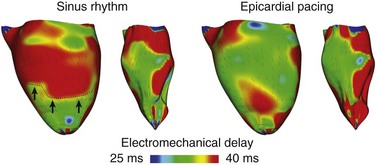
Figure 36-3 Electromechanical delay during sinus rhythm and epicardial pacing in a model of rabbit ventricular electromechanics. Each panel presents the left ventricular (LV) lateral view of epicardium (left) and endocardium (right). The lines represent fiber directions. (Images modified with permission from Gurev V, Lee T, Constantino J, et al: Models of cardiac electromechanics based on individual hearts imaging data: Image-based electromechanical models of the heart. Biomech Model Mechanobiol 10:295–306, 2011.)

The heart achieves an efficient coordinated contraction via a complex network of feedback mechanisms. Organ-level electromechanical modeling by Niederer and Smith ²⁶ explored how cellular-level behaviors affect work transduction, stress and strain homogeneity at the whole-ventricle level, and the feedback loops that regulate normal contraction in an electromechanical model of the rat LV. The simulation research demonstrated that length-dependent changes in Ca sensitivity and the filament overlap, which is believed to constitute the Frank-Starling law, were the two dominant regulators of the efficient transduction of work. The absence of either mechanism not only altered the spatial distribution of stress and strain, but also determined the transmural variation in work. These results showed that feedback from muscle length to tension generation at the cellular level is an important control mechanism of the pumping efficiency of the heart. In a recent study, Land et al²⁷ developed a murine model of electromechanics to explore how length-dependent and velocity-dependent feedback mechanisms alter the pressure developed by the ventricles. Simulation results revealed that the length-dependent changes in Ca sensitivity and filament overlap are the principal regulators of ejection and isovolumetric relaxation. The model also revealed that including velocity dependence of tension in the model extended the LV pressure plateau, resulting in a better match between experiment and simulation. These two studies illustrate the importance of the cellular feedback mechanisms in regulating the emergent electromechanical activity of the whole heart.

Mechanoelectrical Coupling

One of the most important mechanisms of mechanoelectrical coupling in the heart is seen in the sarcolemmal channels that are activated by mechanical stimuli. Of these, stretch-activated channels (SACs) have long been implicated as important contributors to the proarrhythmic substrate in the heart. The nonuniform distribution of positive myofiber strain (stretching) during mechanical contraction under a variety of pathologic conditions could produce, via SACs, proarrhythmic dispersion in electrophysiological properties. SACs have been shown to shorten or lengthen the action potential duration (APD) of a single myocyte or to produce ectopic beats, depending on the timing of the mechanical stimulus application relative to the phase of the action potential. However, uncovering the mechanisms by which SACs contribute to ventricular arrhythmogenesis under a variety of pathologic conditions has been hampered by the lack of experimental methods that can record the 3D electrical and mechanical activity simultaneously and with high spatiotemporal resolution. Thus, computer simulations have emerged as a valuable tool in dissecting the mechanisms by which SACs contribute to arrhythmogenesis.

Role of Mechanoelectrical Feedback in the Stability of Ventricular Tachycardia/Fibrillation

A study by Keldermann et al ²⁸ employed an electromechanical model of human LV to study the effect of mechanoelectrical feedback via SAC on reentrant wave dynamics. SAC conductance was dependent on the stretch ratio in the fiber direction. The authors found that nonuniform activation of SACs can result in the degeneration of a stable scroll wave (representing ventricular tachycardia [VT]) into turbulent patterns characteristic of ventricular fibrillation (VF). Simulation results revealed that regions of wavebreak were those undergoing stretch. At these regions, depolarization due to SAC opening blocked propagation at the stretched region. This simulation study suggested an explanation of the degeneration of ventricular tachycardia into ventricular fibrillation that offered an alternative to the restitution hypothesis. However, Keldermann et al analyzed only how opening of SACs with a reversal potential close to zero and large conductance affected the stability of VT/VF. Because experimental studies have found that SACs exhibit a variety of reversal potentials and conductances,²⁹ a more comprehensive study of the effects of SACs on the stability of VT/VF was needed.

Hu et al ³⁰ aimed to analyze spiral wave stability using an MRI-based electromechanical model of the human heart that included a variety of SAC reversal potentials and channel conductances. Investigators found that recruitment of SACs can also have the opposite effect: Opening of SACs with large negative reversal potentials or of those with reversal potentials close to zero and low conductance led to suppression of scroll wave breakup. As shown in Figure 36-4, A, in a model without SAC representation, scroll waves break up continuously, sustaining VF. Representing SAC with negative reversal potentials (e.g., −60 mV) decreased the average number of scroll wave filaments by 46% to 62%. Mechanistic analysis revealed that recruitment of SACs in this case inhibited scroll wave breakup through flattening of the APD restitution relationship, although to a different degree in different regions. Opening of SACs with less negative reversal potentials (e.g., −10 mV) and with low channel conductances also suppressed scroll wave breakup (Figure 36-4, B) but by a different mechanism, rendering the conduction velocity restitution curve shallower. This study revealed that recruitment of SACs affects scroll wave stability via different mechanisms, depending on the SAC population characteristics.

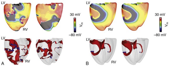
Figure 36-4 Recruitment of stretch-activated channel (SAC) and scroll wave stability. Epicardial transmembrane potential distribution maps on the posterior wall (top) and corresponding semitransparent view of the ventricles (bottom) at two different time points (1 s apart) from a simulation of ventricular fibrillation without SAC representation (A) and a simulation of spiral wavebreak suppression resulting from SAC opening (B). Pink dots in transmembrane potential maps indicate the locations of epicardial phase singularities. Blue denotes filament distribution in the semitransparent view of the ventricles; activation wavefronts are shown in red.

Role of Mechanoelectrical Feedback in Initiation and Perpetuation of Atrial Fibrillation

Because atrial dilatation increases vulnerability to atrial fibrillation (AF), understanding the mechanism for initiation and perpetuation of AF during acute stretch is of paramount importance. The study by Kuijpers et al ³¹ addressed this issue by developing an image-based model of atrial electromechanics. In this model, the mechanical problem was represented by interconnected segments, each consisting of elastic and contractile components, rather than continuum mechanics equations. The model incorporated mechanoelectrical feedback via SAC opening. Simulation results revealed that regional differences in the stretch ratio resulted in heterogeneities in membrane excitability, impulse propagation, APD, and the effective refractory period (ERP). Dispersions of APD and ERP were further enhanced by contraction of active parts of the atria and passive stretch of the rest. The study by Kuijpers et al provided evidence that mechanoelectrical feedback during atrial dilatation resulted in regional changes in electrophysiological properties of the atria, contributing to the inducibility and perpetuation of AF.

Spontaneous Induction of Arrhythmias in the Regionally Ischemic Heart

In the normal heart, tissue stretch can result in spontaneous firing of myocytes and ventricular premature beats (VPBs). In cases of significant mechanical stimuli, such as impact to the precordial region of the chest, as often occurs in normal young athletes, tissue stretch can lead to arrhythmia induction, a phenomenon known as commotio cordis.

In the acutely ischemic heart, occurrence of VPBs has also been associated with rapid regional distention. The mechanisms by which ischemia-induced mechanical dysfunction can result in VPBs and induce reentry were examined by Jie et al.³² A 3D electromechanical model of the beating rabbit ventricles with regional ischemia (4 minutes post occlusion) was developed and contained a central ischemic zone (CIZ), a border zone (BZ), and a normal zone (NZ). In both BZ and CIZ, cells underwent significant stretch during contraction, which led to depolarizations due to the opening of SACs there, while such depolarizations were absent in NZ. The depolarizations resulted in mechanically induced VPBs originating from the ischemic border (particularly in the LV endocardium, where fiber strain and strain rate were the largest), but not from CIZ, although the magnitude of the depolarizations was larger there, because in the latter, ischemic injury suppressed excitability. VPBs then traveled intramurally until emerging from the ischemic border on the epicardium, initiating reentry (Figure 36-5). The study by Jie et al³² provided the first evidence that mechanically induced membrane depolarizations and their spatial distribution within the ischemic region are possible mechanisms by which mechanical activity contributes to the origin of spontaneous arrhythmias.

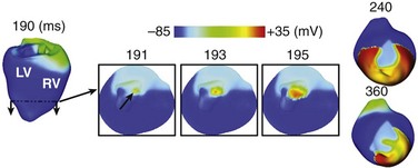
Figure 36-5 Evolution of a mechanically induced ventricular premature beat (VPB) and reentry in the regionally ischemic heart. Insets of 191 to 195 ms present short- and long-axis views of the apical region for better visualization of the spontaneous generation of a propagating wave. 240- to 360-ms panels present a titled anterior view of the ventricles to allow visualization of reentry formation. Arrow in 191-ms inset indicates the location of earliest spontaneous firing. (Images modified with permission from Jie X, Gurev V, Trayanova N: Mechanisms of mechanically induced spontaneous arrhythmias in acute regional ischemia. Circ Res 106:185–192, 2010.)

The role of mechanoelectrical feedback via SACs in altering the electrical activity in myocardial infarction has also been explored using electromechanical modeling. Wall et al ³³ developed an electromechanical model of the infarcted ovine LV and found that APD dispersion in the border zone, which may provide the substrate for arrhythmias in the setting of myocardial infarction, was created by the combined effects of stretch and reduced electrical connectivity.

Cardiac Resynchronization Therapy

Mechanisms Regulating Pump Dyssynchrony and the Response to Cardiac Resynchronization Therapy

Heart failure patients often exhibit contractile dyssynchrony due to electrical intraventricular delay, which diminishes the heart systolic function. Cardiac resynchronization therapy (CRT) is a clinical treatment that re-coordinates contraction by applying appropriately timed pacing stimuli to the ventricles. Although CRT reduces morbidity and mortality, 30% of patients fail to respond to the therapy. Current dyssynchrony indices used to identify potential responders to CRT have poor predictive capability, reflecting an incomplete understanding of the electromechanical behavior involved in dyssychronous heart failure. Ventricular electromechanical simulations offer an opportunity to elucidate the mechanisms that underlie heart failure dyssynchrony and to provide novel therapeutic strategies.

Kerckhoffs et al ³⁴ employed a computational model of failing canine ventricles to assess the sensitivity of current clinical indices quantifying mechanical dyssynchrony to various abnormalities responsible for contractile dysfunction. These indices include the echocardiography-based metric, the time to peak shortening (WTpeak), and the MRI-based metrics of circumferential uniformity ratio estimate (CURE) and internal stretch fraction (ISF), which measure regional strain magnitudes. The abnormalities examined were dilatation, dyssychronous activation, decreased inotropy, and prolonged relaxation. A sensitivity analysis of these abnormalities revealed that all indices were sensitive to dyssychronous activation; however, the synergistic effect of dyssychronous activation and dilatation resulted in greatest changes in ISF and CURE. These simulation results also demonstrated that ISF and CURE were better indices of mechanical dyssynchrony because of their sensitivity to regional strain inhomogeneity. The study concluded that if geometry and electrical activation sequence, which can be established by a clinical evaluation, are the major determinants of regional cardiac function, and if the hard-to-measure material properties play a minor role, patient-specific simulations are feasible and could be performed to suggest optimal CRT strategies tailored to the individual.

Using an electromechanical model of the human ventricles, Niederer et al ³⁵ performed a parameter sensitivity analysis to determine the mechanisms that regulate CRT response. The simulation research revealed that the degree of length dependence on tension and the minimum length of tension generation (the length at which no active tension is generated) were the significant parameters that determined CRT efficacy. At baseline (pre-CRT), attenuating length-dependent tension regulation augmented dyssynchrony in tension development, fiber shortening, and dispersion time to the peak in tension development rate (t_peak). Because synchronization of t_peak following CRT was greatest when length dependence was reduced, the change in the maximum rate of change in LV pressure (CRT response) was the largest. Because the minimum length of tension generation is unaltered in heart failure, these results suggest that reduced length dependence of tension is a mechanism underpinning CRT efficacy.

Optimizing the Response to CRT

Suboptimal placement of the LV lead constitutes a major reason underlying the high nonresponse rate to CRT. To date, no clear consensus has been reached as to where the LV pacing lead should be placed to achieve optimal CRT response. Studies have indicated that the site of latest electrical or latest mechanical activation is associated with greater hemodynamic benefit in CRT; however, recent human data ³⁶ suggest a lack of concordance between the site of latest electrical or mechanical activation and the CRT response.

Constantino et al ³⁷ proposed a new strategy to determine the LV pacing location that optimizes the response to CRT: targeting the regions with the longest electromechanical delay. An MRI-based electromechanical model of canine dyssychronous heart failure (DHF), which incorporated DHF-associated remodeling aspects such as altered ventricular structure, slowed conduction, deranged calcium handling, and reduced stiffness, was employed. CRT was delivered by pacing at the RV apex, with the LV pacing electrode placed at 18 different epicardial sites along the LV free wall. With the use of transmural electromechanical delay maps (Figure 36-6, A), the region with the longest electromechanical delay during left bundle branch block was determined to be the endocardial surface of the lateral wall between the base and the midventricles. Figure 36-6, B presents CRT response as a function of LV pacing location. Maximal hemodynamic benefit occurred when the LV pacing site was located near the base, which was within the region of longest electromechanical delay. The relationship between LV pacing location relative to the longest electromechanical delay region and the corresponding CRT response is quantified in Figure 36-6, C. Improvement in maximal rate of change in LV pressure strongly correlated with the longitudinal distance between the LV pacing site and the center of the region with longest electromechanical delay. This study proposed a new approach to determining the optimal CRT pacing location that accounts for the relation between electrical and mechanical activation sequences in the DHF heart.

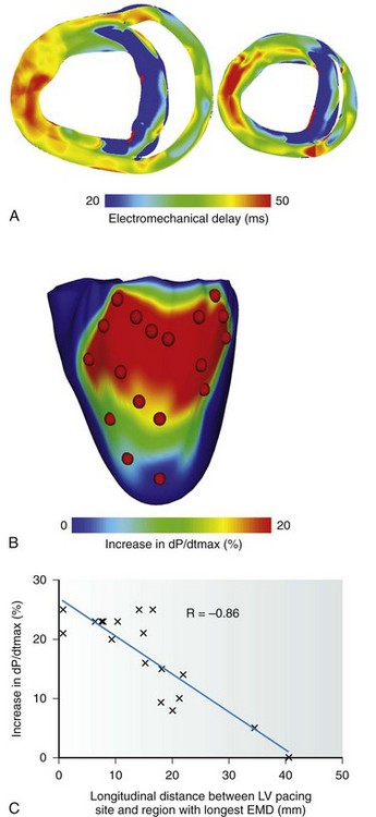
Figure 36-6 Optimization of cardiac resynchronization therapy (CRT) response based on electromechanical delay distribution. A, Transmural short-axis electromechanical delay maps during left bundle branch block generated with a magnetic resonance imaging (MRI)-based electromechanical model of dyssynchronous heart failure. In each map, the anterior and posterior walls are at the top and bottom, respectively. B, Map of the percentage increase in maximal rate of change in pressure as a function of the left ventricular (LV) pacing site. Red dots denote LV pacing sites. C, Correlation of longitudinal distance between LV pacing site and region with longest electromechanical delay, and percentage increase in dP/dtmax. (Images modified with permission from Constantino J, Hu Y, Trayanova N: A computational approach to understanding the electromechanical activation sequence in the normal and failing heart, with translation to the clinical practice of CRT. Prog Biophys Mol Biol. 110:372–379, 2012)

Alternatively, computational models can be used to test new pacing protocols in efforts to optimize CRT. Multi-site CRT, which applies pacing stimuli via one RV lead and two LV leads, has been shown to hold great promise as an alternative strategy in improving CRT response. In addition, quadripolar leads, in which two pacing stimuli can be delivered from one lead, have recently been developed. Niederer et al ³⁸ aimed to determine whether multi-site CRT with a quadripolar lead resulted in improved CRT response in a model of human electromechanics. The study found that multi-site CRT conferred a greater improvement in dP/dtmax, as compared with conventional CRT, only in hearts with an infarct. Because the presence of scar often results in poor CRT response, multi-site CRT with quadripolar leads may thus improve the response to CRT in ischemic cardiomyopathy patients. These studies provide convincing evidence that cardiac electromechanical models can be used for model-guided optimization of CRT lead position and pacing protocols in the near future.

Abnormal Mechanical Deformation and Its Role in Vulnerability to Electrical Shocks and Defibrillation

Clinical studies have demonstrated that patients with dilated, volume- or pressure-overloaded hearts have elevated defibrillation thresholds (DFTs). The mechanisms underlying these findings are not well understood. Using a rabbit ventricular electromechanics model, Trayanova et al ³⁹ conducted simulations of vulnerability to strong shocks and defibrillation under conditions of LV dilatation, and determined the mechanisms by which mechanical deformation may lead to increased vulnerability and elevated DFT. Studies of defibrillation mechanisms have demonstrated that following shock delivery, ventricular geometry and fiber orientation determine the large-scale distribution and magnitude of the virtual electrode polarization (VEP) induced by the strong shock.⁴⁰ Thus, ventricular dilatation could affect VEP through changes in ventricular geometry and fiber architecture, leading to changes in the upper limit of vulnerability and DFT. The model revealed that LV dilatation indeed results in geometric alterations, with the most prominent change noted in septal fiber orientation (Figure 36-7, A). Transmembrane voltage maps following shock application, shown in Figure 36-7, B,C for the undeformed and dilated ventricles, respectively, illustrate the different postshock responses in the two cases. At the end of the shock (see Figure 36-7, B, C; 10 ms), VEP in the bulk of the septal myocardium was different: A larger excitable gap was seen. Consequently, although no reentrant activity was observed in the undeformed ventricles (see Figure 36-7, B), a postshock sustained reentry was formed on the RV side of the septum in the deformed ventricles (see Figure 36-7, C), indicating increased vulnerability to electrical shocks. Similarly, DFT in the dilated ventricles was found to be 38%±20% higher than that in the normal ventricles (for an implantable cardioverter-defibrillator [ICD] electrode configuration), which showed good agreement with experimental findings. Results of the study suggest that not only ventricular geometry but rather rearrangement of fiber architecture in the deformed ventricles is responsible for the increased vulnerability to electrical shocks and for reduced defibrillation efficacy in the dilated ventricles.

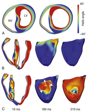
Figure 36-7 A, Short-axis view of ventricular geometry and fiber helix angle for undeformed (left) and dilated (right) rabbit ventricles. Transmembrane potential distributions in the undeformed (B) and dilated (C) ventricles following a monophasic truncated exponential shock of 10-ms duration applied at 120 ms after the last pacing stimuli. This electrode configuration results in a uniform electrical field; thus virtual electrode polarization (VEP) formation depends only on ventricular geometry and fiber orientation. Shock-end transmembrane potential distribution is at 10 ms. Differences in VEP are marked by black ovals. The postshock reentry is illustrated in the 180- and 210-ms panels. (Images modified with permission from Trayanova N, Gurev V, Constantino J, et al: Mathematical models of ventricular mechano-electric coupling and arrhythmia. In Kohl P, Sachs F, Franz MR (eds): Cardiac Mechano-electric Feedback and Arrhythmias. Oxford, 2011, Oxford University Press, pp 256–258.)

Initial Efforts Toward Patient-Specific Electromechanical Modeling of the Heart

With advancements in computational techniques and medical imaging and image processing, the groundwork for patient-specific modeling of electromechanics has been laid, and the era of personalized computational cardiac medicine is fast approaching. The first step in conducting patient-specific cardiac electromechanical simulations is to construct the computational model of the heart from the patient’s medical images. In addition to the challenges involved in reconstructing heart geometry from in vivo clinical scans of low resolution for any other applications, a specific hurdle in constructing the geometric mesh of a patient’s heart for electromechanical applications is defining the unloaded state of the heart, because the heart is constantly loaded during image acquisition. Aguado-Sierra et al ⁴¹ used an iterative estimation scheme to approximate the unloaded geometry from end-diastolic geometry and ventricular pressures. To help accelerate the clinical adoption of personalized simulations, Lamata et al¹⁶ developed a robust method that uses a variation of the warping technique to accurately and quickly construct patient-specific meshes from a template heart in a matter of minutes. Last, the patient’s fiber and sheet orientation needs to be incorporated into the model. To date, no imaging method can obtain the fiber/sheet architecture from in vivo images. Hence, the first patient-specific electromechanical models have incorporated fiber orientations adapted from animal hearts or have used rule-based methods¹⁷ to assign the fiber orientation. Image transformation algorithms for fiber estimation from in vivo hearty scans have shown significant promise.¹⁸ An example of patient fiber orientation estimated with such image transformation algorithms is shown in Figure 36-8, A.

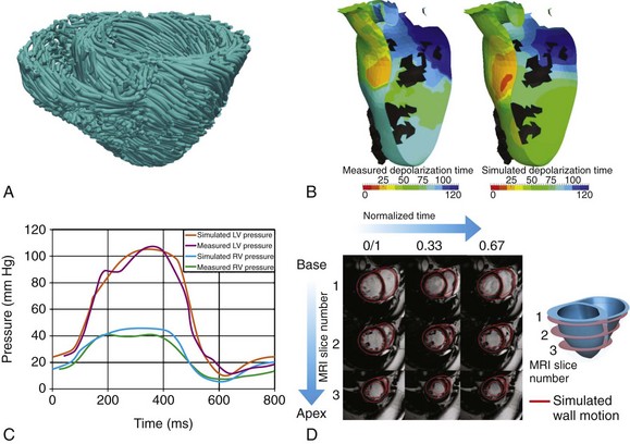
Figure 36-8 Patient-specific electromechanical modeling of the heart. A, Mapping. B, Measured (left) and simulated (right) endocardial ischronal maps of electrical activation with a patient-specific model. C, Left and right ventricular pressure traces from clinical measurements and a patient-specific model. D, Ventricular wall motion (red lines) simulated by a patient-specific model superimposed on the patient’s cineMRI. (A, Modified with permission from Vadakkumpadan F, Arevalo H, Ceritoglu C, et al: Image-based estimation of ventricular fiber orientations for personalized modeling of cardiac electrophysiology. IEEE Trans Med Imaging 31:1051–1060, 2012. B, Modified with permission from Sermesant M, Chabiniok R, Chinchapatnam P, et al: Patient-specific electromechanical models of the heart for the prediction of pacing acute effects in CRT: A preliminary clinical validation. Med Image Anal 16:201–215, 2012. C, Modified with permission from Aguado-Sierra J, Krishnamurthy A, Villongco C, et al: Patient-specific modeling of dyssynchronous heart failure: A case study. Prog Biophys Mol Biol 107:147–155, 2011. D, Modified with permission from Niederer SA, Plank G, Chinchapatnam P, et al: Length-dependent tension in the failing heart and the efficacy of cardiac resynchronization therapy. Cardiovasc Res 89:336–343, 2011.)

Equally important is the process of parameterizing and enriching the electromechanical model of the heart with the patient’s own clinical data. Validating the model with patient-specific metrics personalizes the model and establishes its predictive capabilities. The types of electrophysiological data typically used for clinical validation are the standard ECG, total electrical activation time, and activation maps determined from endocardial recordings. Figure 36-8, B shows measured and simulated isochronal maps of ventricular electrical activation from a patient-specific electromechanical model by Sermesant et al.⁴² To personalize the mechanical problem of the patient’s model heart, the simulation data are compared with pressure and volume curves and gross wall motion from cineMRI. Temporal traces of LV and RV pressures from a patient-specific electromechanical heart model by Aguado-Sierra et al⁴¹ are presented in Figure 36-8, C, and a comparison of cineMRI data with simulated wall motion as calculated from a patient-specific heart model by Niederer et al³⁵ is shown in Figure 36-8, D. In these models, the material properties of the myocardium and parameters of the myofilament model have been systematically adjusted to achieve match between measured and simulated results. These initial results in the development of patient-specific cardiac electromechanical models attest to the potential utility of cardiac simulation in the diagnosis and treatment of disorders in the pumping function of the heart.

References

1. Plank, G, Zhou, L, Greenstein, JL, Cortassa, S, et al. From mitochondrial ion channels to arrhythmias in the heart: Computational techniques to bridge the spatio-temporal scales. Philos Transact A Math Phys Eng Sci. 2008; 366:3381–3409.
2. Noble, D, Rudy, Y. Models of cardiac ventricular action potentials: Iterative interaction between experiment and simulation. Philos Transact A Math Phys Eng Sci. 2001; 359:1127–1142.
3. Trayanova, NA, Rice, JJ. Cardiac electromechanical models: From cell to organ. Front Physiol. 2011; 2:43.
4. Nordsletten, DA, Niederer, SA, Nash, MP, et al. Coupling multi-physics models to cardiac mechanics. Prog Biophys Mol Biol. 2011; 104:77–88.
5. Holzapfel, GA, Ogden, RW. Constitutive modelling of passive myocardium: A structurally based framework for material characterization. Philos Transact A Math Phys Eng Sci. 2009; 367:3445–3475.
6. Vetter, FJ, McCulloch, AD. Three-dimensional analysis of regional cardiac function: A model of rabbit ventricular anatomy. Prog Biophys Mol Biol. 1998; 69:157–183.
7. Stevens, C, Remme, E, LeGrice, I, et al. Ventricular mechanics in diastole: Material parameter sensitivity. J Biomech. 2003; 36:737–748.
8. Legrice, IJ, Hunter, PJ, Smaill, BH. Laminar structure of the heart: A mathematical model. Am J Physiol. 1997; 272:H2466–H2476.
9. Vadakkumpadan, F, Arevalo, H, Prassl, AJ, et al. Image-based models of cardiac structure in health and disease. Wiley Interdiscip Rev Syst Biol Med. 2010; 2:489–506.
10. Gurev, V, Lee, T, Constantino, J, et al. Models of cardiac electromechanics based on individual hearts imaging data: Image-based electromechanical models of the heart. Biomech Model Mechanobiol. 2011; 10:295–306.
11. Bishop, MJ, Plank, G, Burton, RA, et al. Development of an anatomically detailed mri-derived rabbit ventricular model and assessment of its impact on simulations of electrophysiological function. Am J Physiol Heart Circ Physiol. 2010; 298:H699–H718.
12. Helm, PA, Tseng, HJ, Younes, L, et al. Ex vivo 3D diffusion tensor imaging and quantification of cardiac laminar structure. Magn Reson Med. 2005; 54:850–859.
13. McDowell, KS, Vadakkumpadan, F, Blake, RC, et al. Methodology for patient-specific modeling of atrial fibrosis as a substrate for atrial fibrillation. J Electrocardiol. 2012; 45:640–645.
14. Nickerson, D, Smith, N, Hunter, P. New developments in a strongly coupled cardiac electromechanical model. Europace. 2005; 7(suppl 2):118–127.
15. Prassl, AJ, Kickinger, F, Ahammer, H, et al. Automatically generated, anatomically accurate meshes for cardiac electrophysiology problems. IEEE Trans Biomed Eng. 2009; 56:1318–1330.
16. Lamata, P, Niederer, S, Nordsletten, D, et al. An accurate, fast and robust method to generate patient-specific cubic hermite meshes. Med Image Anal. 2011; 15:801–813.
17. Bayer JD, Blake RC, Plank G, Trayanova NA: A novel rule-based algorithm for assigning myocardial fiber orientation to computational heart models. Ann Biomed Eng. In press.
18. Vadakkumpadan, F, Arevalo, H, Ceritoglu, C, et al. Image-based estimation of ventricular fiber orientations for personalized modeling of cardiac electrophysiology. IEEE Trans Med Imaging. 2012; 31:1051–1060.
19. Trayanova, NA. Whole-heart modeling: Applications to cardiac electrophysiology and electromechanics. Circ Res. 2011; 108:113–128.
20. Land, S, Niederer, SA, Smith, NP. Efficient computational methods for strongly coupled cardiac electromechanics. IEEE Trans Biomed Eng. 2012; 59:1219–1228.
21. Provost, J, Gurev, V, Trayanova, N, et al. Mapping of cardiac electrical activation with electromechanical wave imaging: An in silico-in vivo reciprocity study. Heart Rhythm. 2011; 8:752–759.
22. Provost, J, Lee, WN, Fujikura, K, et al. Imaging the electromechanical activity of the heart in vivo. Proc Natl Acad Sci U S A. 2011; 108:8565–8570.
23. Kerckhoffs, RC, Bovendeerd, PH, Kotte, JC, et al. Homogeneity of cardiac contraction despite physiological asynchrony of depolarization: A model study. Ann Biomed Eng. 2003; 31:536–547.
24. Usyk, TP, McCulloch, AD. Relationship between regional shortening and asynchronous electrical activation in a three-dimensional model of ventricular electromechanics. J Cardiovasc Electrophysiol. 2003; 14:S196–S202.
25. Gurev, V, Constantino, J, Rice, JJ, et al. Distribution of electromechanical delay in the heart: Insights from a three-dimensional electromechanical model. Biophys J. 2010; 99:745–754.
26. Niederer, SA, Smith, NP. The role of the Frank-Starling law in the transduction of cellular work to whole organ pump function: A computational modeling analysis. PLoS Comput Biol. 2009; 5:e1000371.
27. Land, S, Niederer, S, Aronsen, JM, et al. An analysis of deformation-dependent electromechanical coupling in the mouse heart. J Physiol. 2012; 590(Pt 18):4553–4569.
28. Keldermann, RH, Nash, MP, Gelderblom, H, et al. Electromechanical wavebreak in a model of the human left ventricle. Am J Physiol Heart Circ Physiol. 2010; 299:H134–H143.
29. Hu, H, Sachs, F. Stretch-activated ion channels in the heart. J Mol Cell Cardiol. 1997; 29:1511–1523.
30. Hu Y, Gurev V, Constantino J, et al: Novel mechanisms for the suppression of scroll wave breakup via mechano-electric feedback. In preparation.
31. Kuijpers, NH, Potse, M, van Dam, PM, et al. Mechanoelectrical coupling enhances initiation and affects perpetuation of atrial fibrillation during acute atrial dilation. Heart Rhythm. 2011; 8:429–436.
32. Jie, X, Gurev, V, Trayanova, N. Mechanisms of mechanically induced spontaneous arrhythmias in acute regional ischemia. Circ Res. 2010; 106:185–192.
33. Wall, ST, Guccione, JM, Ratcliffe, MB, et al. Electromechanical feedback with reduced cellular connectivity alters electrical activity in an infarct injured left ventricle: A finite element model study. Am J Physiol Heart Circ Physiol. 2012; 302:H206–H214.
34. Kerckhoffs, RC, Omens, JH, McCulloch, AD, et al. Ventricular dilation and electrical dyssynchrony synergistically increase regional mechanical nonuniformity but not mechanical dyssynchrony: A computational model. Circ Heart Fail. 2010; 3:528–536.
35. Niederer, SA, Plank, G, Chinchapatnam, P, et al. Length-dependent tension in the failing heart and the efficacy of cardiac resynchronization therapy. Cardiovasc Res. 2011; 89:336–343.
36. Spragg, DD, Dong, J, Fetics, BJ, et al. Optimal left ventricular endocardial pacing sites for cardiac resynchronization therapy in patients with ischemic cardiomyopathy. J Am Coll Cardiol. 2010; 56:774–781.
37. Constantino, J, Hu, Y, Trayanova, N. A computational approach to understanding the electromechanical activation sequence in the normal and failing heart, with translation to the clinical practice of CRT. Prog Biophys Mol Biol. 2012; 110:372–379.
38. Niederer, SA, Shetty, AK, Plank, G, et al. Biophysical modeling to simulate the response to multisite left ventricular stimulation using a quadripolar pacing lead. Pacing Clin Electrophysiol. 2012; 35:204–214.
39. Trayanova, N, Gurev, V, Constantino, J, et al, Mathematical models of ventricular mechano-electric coupling and arrhythmia OxfordKohl P, Sachs F, Franz MR, eds. Cardiac Mechano-electric Feedback and Arrhythmias. 2011:256–258.
40. Trayanova, N, Constantino, J, Ashihara, T, et al. Modeling defibrillation of the heart: Approaches and insights. IEEE Rev Biomed Eng. 2011; 4:89–102.
41. Aguado-Sierra, J, Krishnamurthy, A, Villongco, C, et al. Patient-specific modeling of dyssynchronous heart failure: A case study. Prog Biophys Mol Biol. 2011; 107:147–155.
42. Sermesant, M, Chabiniok, R, Chinchapatnam, P, et al. Patient-specific electromechanical models of the heart for the prediction of pacing acute effects in CRT: A preliminary clinical validation. Med Image Anal. 2012; 16:201–215.