MULTIPLANAR REFORMATION

MPR refers to the reconstruction of three-dimensional data into a new orientation. For example, a volumetric CTA data set acquired in the axial plane can be reconstructed for viewing in a coronal plane or a plane of any obliquity using MPR. MPR images can be reconstructed into linear (e.g., coronal, sagittal, axial, oblique; Figs. 83-1 and 83-2) or curved plane images (Fig. 83-3). The process does not change the original data or voxels. In the MPR process, interpolation is needed to rearrange data into a different coordinate system. Curved reformatting is useful for viewing tortuous vessels such as the coronary arteries on CTA because it unravels the tortuous segments for linear viewing of the vessel (i.e., straightens out the vessel in length). It is particularly useful for showing vascular detail in cross-sectional profile along the vessel length, facilitating characterization of stenoses or other intraluminal abnormalities. The pitfall is that manual definition of curved planes may not be accurate for actual measurements and is potentially a time-consuming process because operator interaction is often required. Automated curve detection methods can expedite processing but fail if there are image artifacts within the data (e.g., motion blurring or high-value nonvascular structures such as calcium on CTA). These may be erroneously labeled as vessel lumen, thereby introducing inaccurate curved vascular lumen reformation.

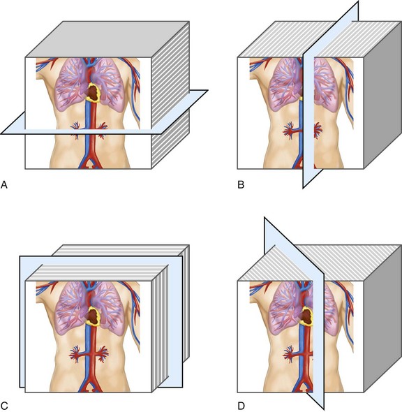
FIGURE 83-1 Multiplanar reformation (MPR). A, The diagram represents a stack of axial images that can be reconstructed and interpolated to a three-dimensional volume. Sagittal (B) and coronal (C) MPR views can be sampled and generated from it. D, It can also be sampled in an arbitrary oblique MPR view, which can be used for improved visualization of specific vascular segments.

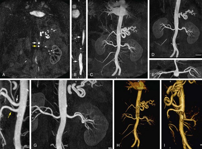
FIGURE 83-2 Normal renal contrast-enhanced three-dimensional MPR. With MPR, a single-voxel view of the three-dimensional data set can be individually visualized. A, On the coronal MPR, the celiac trunk (white arrow) and superior mesenteric artery (yellow arrow) are seen but their relationship to the renal arteries and aorta is not evident because the coronal MPR does not include these structures. B, Similarly, on a sagittal MPR, only a portion of the abdominal aorta (arrows) is included on this coronal MPR obtained at the edge of the abdominal aorta. C, On a whole-volume coronal MIP, the renal arteries and their origin from the abdominal aorta are much more clearly viewed than on the thin single-voxel MPR. On subvolume MIP (D, coronal; E, axial; F, sagittal; G, oblique coronal), overlapping structures can be excluded from the slab to visualize the renal arteries preferentially. F, On the sagittal subvolume MIP, the origins of the celiac trunk (white arrow) and superior mesenteric artery (yellow arrow) can be clearly seen arising anteriorly from the abdominal aorta. On VR (H, coronal; I, oblique sagittal), the observer is provided with improved depth perception of the abdominal aorta and renal arteries compared with MIP images (compare H with C).

FIGURE 83-3 Normal coronary CTA. Lower right images, The proximal left anterior descending (LAD) coronary artery (arrows) is well seen on curved MPR. Top right image, Cross section of the proximal LAD is shown. Left, Actual green line tracing used to predict the curved MPR on a VR projection of the coronary CTA. Ao, aortic root.

Nearest Neighbor Interpolation

Interpolation is an important concept in the context of image reconstruction. As demonstrated in Figure 83-4, a slice of an original acquired image is composed of known data points. In this example, the circles are known data grids. Triangles are points that need to be interpolated because of MPR needs. The left known data signal intensity (SI) value is SI_a = 100, and right known signal intensity value is SI_b = 100. The simplest interpolation is the nearest neighbor. In nearest neighbor interpolation, the new interpolated data point (i.e., triangle) is closer to the right data point, where SI_b is, so the unknown interpolated signal intensity (SI_i) is set to be the same as SI_b, that is, SI_i.

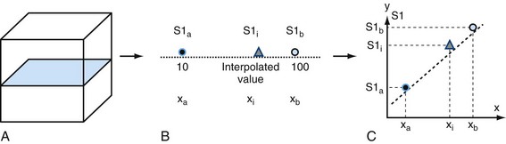
FIGURE 83-4 Multiplanar reformation. A, A slice of the original acquired image composed of known data points. B, Example of two known grids with an oblique line that are defined by oblique MPR. Circles are data grids that are known. Triangles are points that need to be interpolated because of MPR needs. C, Explanation in SI – x coordinate.

MAXIMUM INTENSITY PROJECTION

MIP is another common method for two-dimensional projectional viewing CTA and MRA three-dimensional data. In MIP, the highest signal intensity values are projected from the data encountered by a ray cast through an object to the viewer’s eye (Fig. 83-5). MIP is not averaging the average signal intensities from slice to slice along the projected axis (mean value); instead, it finds the highest value along a projection line and assigns that value to the pixel represented on the two-dimensional projected image. For CTA, the pixel values are in density or Hounsfield units; for MRA, the pixel values are in signal intensity. In this way, three-dimensional data can be collapsed into a two-dimensional projection image (see Fig. 83-2). MIP can be generated using the whole three-dimensional volume or a smaller subvolume (slab, or subvolume MIP; Figs. 83-6 and 83-7).

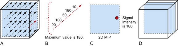
FIGURE 83-5 Maximum intensity projection. A, Three-dimensional MRA data set. The viewer’s eye cast ray projections from front to back into the page. B, One of the projection rays is zoomed in, with signal intensities of 20, 100, 50, 180, and 10. The highest intensity is 180. C, Corresponding projected point on two-dimensional MIP image. A signal intensity of 180 is assigned to that pixel. D, Subvolume MIP that is projected through limited volume, or slab, of the entire three-dimensional data set.

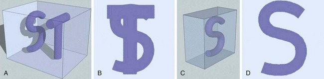
FIGURE 83-6 Subvolume MIP. A, Two parallel three-dimensional objects (letters S and T) will overlap each other on a frontal MIP projection (B) such that the margins of the individual letters overlap and are not distinct. C, On a subvolume MIP, one object (S) can be isolated from the other object (T) and reconstructed so that only the target object will be seen on the subvolume MIP (D).

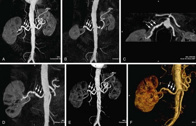
FIGURE 83-7 Renal fibromuscular dysplasia (FMD) on contrast-enhanced three-dimensional MRA. On MIP (A, coronal thick slab; B, coronal thin slab; C, thin slab axial; D, thin slab oblique coronal), the typical string of beads appearance of FMD (arrows) is seen in the mid–right renal artery. Minimizing the target volume on a subvolume MIP allows improved viewing of the three-dimensional data so that overlapping structures can be removed (compare A with B). This is seen also on VR (E, coronal; F, oblique coronal). The improved depth perception is evident on VR (compare F with D).

MIP is useful for projected viewing of CTA and MRA in views similar to conventional x-ray angiograms. MIP images provide the big picture but are often suboptimal for viewing specific segments that are tortuous, such as near vessel origins or bifurcations, where subvolume MIP may be more helpful, especially if there are overlapping vessels such as the celiac artery (Fig. 83-8). Furthermore, because it projects simply brightest value, full-volume or thick MIP processing does not provide depth perception because the three-dimensional data are collapsed for viewing of only the brightest values. Subvolume MIP provides planar viewing of thinner volumes versus single-voxel viewing using MPR but may also mask luminal abnormalities. With MIP, the pitfall is that of a loss in depth information. Therefore, MIP misrepresents anatomic spatial relationships in depth directions. Moreover, MIP shows only the highest intensity along the projected ray. A high-intensity mass such as calcification will obscure information from intravascular contrast material. Vessels with low signal intensity values may be partially or completely imperceptible on MIP images. Alternatively, the bright signal of the lumen may mask subtle detail such as an intimal tear in an arterial dissection.

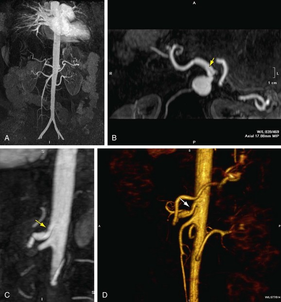
FIGURE 83-8 Celiac artery dissection on contrast-enhanced three-dimensional MRA. A, On coronal thick slab MIP, the celiac dissection is not clearly seen. B, However, on axial subvolume MIP, an intimal flap (arrow) is noted in the proximal celiac artery. C, Sagittal subvolume MIP shows the celiac artery dissection (arrow) as a spiral indentation to the superior surface of the proximal true lumen of the proximal celiac artery. Note that on contrast-enhanced MRA, gadolinium chelate contrast medium fills both the true and false lumen, if patent. In these images, the true lumen (inferior channel) is well seen but there is incomplete filling of the superiorly located false lumen, which results in the appearance of a superior spiral indentation to the proximal celiac artery. D, On oblique sagittal VR, the spiral indentation of the unopacified false channel (arrow) and the intimal flap just distal to the indentation are more clearly demonstrated.

VOLUME RENDERING

Volume rendering (VR) is a visualization technique that represents a three-dimensional CTA or MRA data set (see Figs. 83-2, 83-7, and 83-8) as an opaque or translucent fashion but preserves the depth information of the data set, which is not afforded by MIP reconstruction (Fig. 83-9). It has replaced most imaging applications such as surface rendering, with the notable exception of interior vessel analysis. VR assigns opacity values based on a percentage classification from 0% to 100% using a variety of computational techniques. It uses all acquired data, so it needs greater processing power than the other applications discussed. Once the data have been assigned percentages, each tissue is assigned a color and degree of transparency. Then, by casting simulated rays of light through the volume, VR generates a three-dimensional image. The color used in volume rendering is a pseudocolor, which does not represent the true optical color of the tissues. However, color enhances the human eyes’ ability to perceive depth relationships (see Fig. 83-3). On VR reconstruction, the three-dimensional data can be visualized using various degrees of opacity and transparency, which afford different viewing perspectives of the image data (Fig. 83-10).

FIGURE 83-9 Volume rendering versus maximum intensity projection reconstruction. A, Two three-dimensional objects are shown. If volume rendering is used, the depth information is preserved, thereby showing the relationship between the two objects in a front view (B) or back view (C). However, on MIP reconstruction, separation of the objects (S and T) is not evident because the contours of the objects overlap and blend, making visual separation difficult. On the MIP images (D, front view; E, back view), the contours of both objects blend and it is hard to see the spatial depth relationship (i.e., which is in the foreground versus which is in the background).

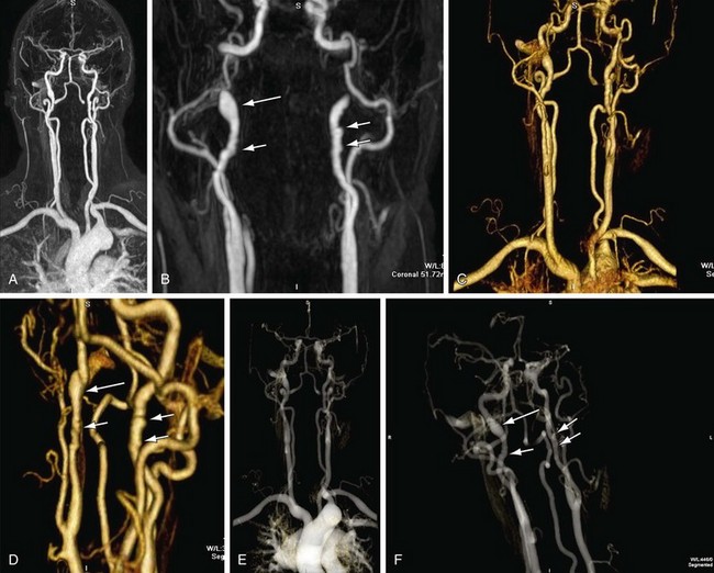
FIGURE 83-10 Bilateral internal carotid artery fibromuscular dysplasia (FMD). A, On thick slab MIP, the string of beads appearance characteristic for FMD is not immediately evident. B, However, on thinner subvolume MIP, the string of beads appearance is seen in both internal carotid arteries (arrows), with an aneurysm (large arrow) in the distal right internal carotid artery. On opaque volume rendered (VR) (C, coronal; D, oblique sagittal), the string of beads (D, arrows) and distal right aneurysm (D, large arrow) is again noted. Similarly on translucent VR views (E, coronal; F, oblique sagittal), the same findings are noted. On translucent VR views, one can see through the vascular structures.

The basic idea of volume rendering is to find the best approximation of the low-albedo volume rendering optical model that represents the relation between the volume intensity and opacity function and the intensity in the image plane. A common theoretical model on which VR algorithms are based is described in equation (2)⁶:

(2)

where α is the opacity samples along the ray and C is the local color values derived from the illumination model. All algorithms obtain colors and opacities in discrete intervals along a linear path and composite them in front to back order. The raw volume densities are used to index the transfer functions for color and opacity; thus, the fine details of the volume data can be expressed in the final image using different transfer functions.

Therefore, there are many adjustable parameters in volume rendering, such as window center, window width, color, transparency, degree of opacity, and shading. Different vendors have different standards for parameters as well as core algorithms for volume rendering, so the appearance of rendered images may vary slightly among vendors.

In the volume rendering process, geometric structures from volume data and render volumes are based on fuzzy or percentage classification and are different from, and generally more useful than, images generated using surface rendering. VR is actually a direct volume-rendering (DVR) method. DVR techniques include ray casting, splatting, shear warp, texture mapping, and hardware-driven volume rendering. Each approach has its own advantages and disadvantages. Shear warp and three-dimensional texture mapping volume rendering are devised to maximize frame rates at the expense of image quality and are used for the assessment of dynamic three-dimensional data sets. Image-aligned splatting and ray casting are devised to achieve high image quality at the expense of performance. A combination of these techniques is possible based on specific applications. However, this discussion is beyond the scope of this basic introductory chapter on three-dimensional postprocessing.

KEY POINTS

Three-dimensional data sets from CTA and MRA can be viewed using a variety of postprocessing tools, most commonly, multiplanar reformation, maximum intensity projection, and volume rendering.

MPR provides reconstructed viewing of three-dimensional data in an arbitrary plane that can be linear (e.g., axial, coronal, sagittal, oblique) or curved.

MIP generates two-dimensional projectional views of the three-dimensional data set and can be performed as a thick full data or thinner slab subvolume reconstruction. Subvolume MIP provides improved ability to isolate and view specific vascular segments.

VR retains image depth information for improved viewing of vascular structures compared with MIP.