Basic Optic Nerve Scan Patterns and Output
▶ Volume scans: these are analogous to macular cube scans in which a volumetric set of data is acquired, centered at the optic nerve head. These may be square or rectangular cubes of data, or cylindrical cubes acquired by circumferential scanning around the optic nerve. The Cirrus HD-OCT scanning protocol acquires a 6 mm × 6 mm cube of data at the optic nerve head using a series of rapid B-scans (200 × 200). Software processing within the SD-OCT machine then identifies the center of the optic disc and creates a 3.46 mm circle centered on this location for registration purposes. The data set is then used to measure retinal nerve fiber layer thickness. The Heidelberg Spectralis volumetric scanning protocols acquire a set of three sequential circular scans, each with 256 axial scans, centered at the optic nerve head. This yields a cylindrical volume with a diameter of 3.4 mm through and around the optic nerve head.
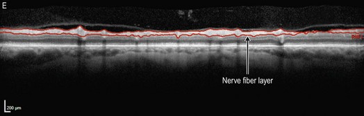
▶ Line Scans: a single or a series of high-resolution B-scans can be obtained through the optic nerve head similar to the line scans obtained in the macula, to allow for higher resolution visualization of structure and pathology at the optic nerve head. Line scans are most frequently used in the qualitative interpretation of data and the identification of anatomic anomalies.
Volume scans obtained through the optic nerve head are processed to delineate the optic disc margin and optic disc surface contour and segmented to obtain the retinal nerve fiber layer (NFL) boundaries. Since most OCT measurements of the optic nerve head are highly sensitive to scan position, all commercially available OCT devices have motion correction software. The information obtained from the optic nerve volumetric scans is processed to obtain the following details.
Retinal Nerve Fiber Layer (RNFL) Thickness
RNFL thickness is calculated by the OCT devices as the distance between the internal limiting membrane and the outer aspect of the NFL (Fig. 5.1.1). Because the RNFL varies with distance from the center of the optic nerve, most machines use a circle of a pre-defined diameter (usually between 3.4–3.46 mm) around the center of the optic nerve as the reference point at which to calculate RNFL thickness. One of the reasons that measurement of the RNFL between machines is not comparable is that different machines use circles of different diameters around the center of the optic nerve head.
Optic Nerve Morphology
The software in various SD-OCT machines also calculates and displays areas for the optic disc, cup and rim, volumes for optic nerve head, cup and rim, cup-to-disc ratios and cup-to-disc horizontal and vertical ratios (Fig. 5.1.2).
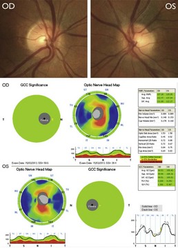
Figure 5.1.2 Composite figure showing the right and left optic disc photographs (top) and OCT printout (bottom) of a normal individual. The optic disc area is 1.53 mm2 and 1.58 mm2 for the right and left optic disc, respectively. For this individual all retinal nerve fiber layer and ganglion cell complex parameters are colored green, indicating the patient is likely normal. The right bottom TSINT graph shows the results from both eyes plotted together. Any statistically significant asymmetry between the two eyes is shown in color between the two lines on the plots.
Ganglion Cell Complex (GCC)
The ganglion cell complex consists of three inner retinal layers: the NFL (formed by axons of the ganglion cells), the ganglion cell layer (cell body of the ganglion cells) and the inner plexiform layer (dendrites of the ganglion cells). The GCC scan is a series of B-scans centered on the macula and quantifies the thickness in all of these three layers. After image processing, GCC thickness is calculated as the distance between the internal limiting membrane and the outer boundary of the inner plexiform layer. The software presents the results as a color-coded ‘map’, which compares the examined eye with a normative database and indicates deviations from the normal values (Figs 5.1.2 and 5.1.3). The GCC scan must be precisely centered at the fovea to have its results compared with a normative database, or to permit progression analysis.
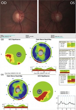
Figure 5.1.3 Composite figure showing the right and left optic disc photographs (top) and OCT printout (bottom) of a patient with glaucoma. Both optic discs show an increase in the cup-to-disc ratio with loss of neuroretinal rim tissue on the inferior aspect of the optic disc. The optic nerve head map shows substantial retinal nerve fiber layer thinning in the inferotemporal sector in both eyes, with a corresponding thinning of the ganglion cell complex in the inferior macula.