[level-membership-for-internal-medicine-category]
Chapter 6 Attenuation/Scatter/Resolution Correction
Physics Aspects
INTRODUCTION
A number of factors can cause artifacts in cardiac single-photon emission computed tomography (SPECT) imaging.1 Among these are the attenuation and scattering of the photons in the patient’s tissues and the finite and distance-dependent spatial resolution SPECT systems. A significant amount of research and development has gone into perfecting clinically robust compensation strategies for these. The present status of clinical trials has led the American Society of Nuclear Cardiology and the Society of Nuclear Medicine to jointly develop and publish a position statement on attenuation correction (AC), which concluded “that the adjunctive technique of attenuation correction has become a method for which the weight of evidence and opinion is in favor of its usefulness.”2 To achieve an improvement in diagnostic accuracy with AC, it is required for physicians to modify their “approach to image interpretation accounting for the effects of these methods on the resultant images,”2 and “use hardware and software that have undergone clinical validation and include appropriate quality-control tools (see Chapter 7).”2
It is our belief this recognition of the utility of AC will be followed by that of the need for also correcting for scatter and distance-dependent spatial resolution. Our position is that the more completely the physics of imaging is correctly included in reconstruction, the more accurate will be the diagnosis from the reconstructed slices. Thus, the goals of this chapter are to (1) provide an introduction to the physics of imaging and how this can be incorporated into reconstruction and (2) illustrate that when this is done, diagnostic accuracy can be improved. Other related reviews on this have been published by Bacharach and Buvat,3 King and colleagues,4,5 Bailey,6 and Zaidi and Hasegawa.7
IMPACT OF ATTENUATION, SCATTER, AND RESOLUTION ON CARDIAC SINGLE-PHOTON EMISSION COMPUTED TOMOGRAPHY (See Chapter 7)
Interactions and Exponential Attenuation
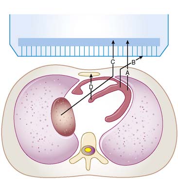
For a photon—whether gamma ray from technetium (99mTc) or x-ray subsequent to the decay of thallium (201Tl)—to become part of a cardiac image, it must first escape the body (see photon A in Fig. 6-1). The chances of this occurring are reduced in proportion to the likelihood that it will interact in the patient’s body before it can escape. At the photon energies of interest in nuclear cardiology, the major interactions in tissues are Compton scattering and photoelectric absorption.8,9 In Compton scattering, a photon interacts with an electron that is loosely bound compared to the photon’s energy. The result of this interaction is the ejection of the electron from the atom and the creation of a new photon having a lower energy and different direction (see photons B and C in Fig. 6-1). The probability of interaction per unit path length (characterized by the linear attenuation coefficient for Compton scattering) depends on the tissue density and number of electrons per gram and decreases slowly with increasing photon energy. In photoelectric absorption, the photon imparts all of its energy to an electron, which is then ejected from the atom. The ejected photoelectron carries a kinetic energy that is equal to the energy of the incident photon minus the binding energy with which it was held to the atom. No scattered photon is emitted in the photoelectric interaction (see photon D in Fig. 6-1). However, characteristic radiation will likely be emitted when the electrons of the atom rearrange to fill the vacancy left by the photoelectron. The linear attenuation coefficient for photoelectric absorption increases as the cube of the atomic number of the atom, depends on tissue density, and decreases as the inverse cube of the photon energy.

where μ is the linear attenuation coefficient (sum of all the coefficients for individual interactions) and x is the thickness of the attenuator the photons pass through. If the attenuator is made up of a number of materials of various compositions, then the product μx in Eq. 1 is replaced by a sum of the attenuation coefficient for each material times the thickness of the material the transmitted photons pass through (path length the photons travel in the material). As a result of the differences in attenuation coefficient with type of tissue, the TF will vary with the materials traversed, even if the total patient thickness between the site of the emission and the camera is the same. Thus, one needs to have patient-specific information on the spatial distribution of attenuation coefficients (an attenuation map) to calculate the attenuation, which decreases the probability of photon detection.
Attenuation Artifacts (See Chapter 6)
The change in TF with direction of the photons and between different locations in the patient results in a variation in attenuation. This can be visualized in planar images as, for example, breast shadows and decreased counts in the presence of an elevated diaphragm. In SPECT slices, these artificial shadows are difficult to recognize; however, there is a pattern of altered relative counts consistent with the influence of attenuation in the mean bull’s eye polar maps of patients with a low likelihood of CAD. Eisner and colleagues reported decreased relative counts in the anterior wall of 201Tl polar maps for females due to breast attenuation, and a relative decrease in the inferior wall of males, which may be due to diaphragmatic attenuation.10 The problem is that the location, extent, and severity of these reduced-count regions vary from patient to patient as a function of their anatomy. Thus, the variation in the pattern of apparent localization in disease-free patients is increased, resulting in more false-positive results (lower specificity) at any given level of true-positive results (sensitivity).
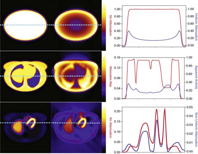
The types of changes in the reconstructed activity distributions when attenuation is present are illustrated in Figure 6-2. The top row of this figure shows what can be expected in the simple case of an elliptically shaped uniform-activity distribution without and with the presence of attenuation caused by a uniform attenuation distribution within the object. Note that attenuation causes a scaling of the reconstructed activity distribution such that there is a decrease by more than a factor of 2 at the outside, and a further decrease as one moves toward the center or most attenuated portion of the distribution. Hence an extended object that has a uniform distribution to begin with would have a loss in uniformity dependent on the relative depths of locations within it. The middle row of the figure shows the more complex case of a uniform source distribution that is attenuated by a non-uniform attenuation distribution simulating that of a cross-section through a female patient. This attenuation distribution and subsequent source and attenuator distributions the employed in the figures of this chapter were obtained from the mathematic cardiac-torso (MCAT) digital anthropomorphic phantom.11 Notice that because the lungs have an attenuation coefficient approximately one-third that of soft tissue, there is now less attenuation within them than would have occurred had the entire cross-section consisted of soft tissues. Thus with attenuation, there appears to be a higher concentration of activity within them than the surrounding soft tissue, when actually the concentration was uniform. Notice also the sharp transition in apparent concentration of activity between the medial boundary of the lung and the heart region. The heart lateral wall is attenuated significantly more than the lung next to it. This explains why AC correction is very sensitive to having the correct registration between emission imaging and attenuation maps. A small movement can cause a big difference in the correction applied. The bottom row shows the even more complex case of both non-uniform source and attenuation distributions from the MCAT phantom simulating that of 99mTc-sestamibi imaging. At the far left, in the absence of attenuation, the distribution of activity within the heart wall is uniform; however, when attenuation is included, a non-uniform distribution results, with the apex and lateral wall being brighter than the deeper lateral wall. Notice also that with attenuation present, there is now a mild change in the size and shape of the heart, as well as a significant distortion of the liver. With attenuation, there now is activity reconstructed as being outside the body. Such geometric distortion is greater for 180-degree reconstruction (as performed for these slices) than 360-degree reconstruction, owing to the greater inconsistencies in the emission profiles in the absence of their averaging by combining conjugate views.12 The positive and negative tails from hot sources, which result from the incomplete cancellation of the inconsistent data in the emission profiles, can also lead to significant distortions in cardiac wall counts when there is significant extracardiac localization, such as with hepatic uptake. Germano and colleagues showed in phantom studies that an apparent reduction in counts occurs with the presence of a “hot” liver in the slices with the heart.13 Nuyts and colleagues14 observed that use of 360 degrees as opposed to 180 degrees with filtered backprojection (FBP) reconstruction reduced the magnitude of the artifact. The artifact was further reduced by use of attenuation compensation with maximum-likelihood expectation-maximization (MLEM) reconstruction.
The artifactual decrease in apparent activity within the heart walls due to nearby extracardiac activity is further illustrated in the short-axis slices and circumferential count profiles at the top of Figure 6-3 for 180-degree reconstruction of Monte Carlo simulations15 of the MCAT phantom.11 The top set of slices are with the liver uptake simulated as the same as that of the background. The next lower set of three slices shows the artifactual decrease in the inferior wall caused by the alteration of the liver activity to be the same as that of the heart. This alteration is illustrated graphically in the plots of the maximum count circumferential count to the right. There, one sees the typical pattern of a decrease in activity in the inferior versus the anterior wall due to the greater depth of the inferior wall, but this difference is dramatically accentuated by the increase in liver activity. This alteration in the apparent distribution of activity within the slices can be understood by the theory of the impact of attenuation on positron emission tomography (PET) and SPECT slices developed by Nuyts et al.,16 Bai et al.,17 and Bai and Shao.18 By this theory, attenuation causes a scaling of the counts at a given position, as illustrated in Figure 6-2, and a shifting of the local counts due to the attenuation of the other activity within the slice. It is this shifting that creates a negative bias that is the cause of the artifactual decrease in the inferior wall of the heart.
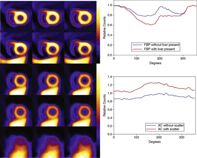
That AC, when included within iterative reconstruction, can correct this artifactual decrease as illustrated in the middle set of three short-axis slices at the left in Figure 6-3, and in the corresponding circumferential profile at the right. Notice that with AC, the wall now becomes fairly uniform in uptake. Notice also that the liver now becomes more intense than the heart, even though they were simulated as having the same concentration of activity. The reason for the apparent difference is the partial volume effect (PVE),9 which causes structures smaller in any dimension than two to three times the full-width-at-half-maximum (FWHM) measure of the system spatial resolution to be blurred such that their apparent activity is less than the actual value.
Broad Beam Attenuation and Scatter
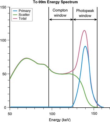
Equation 1 is accurate only (1) for a beam of photons with the same energy and (2) under the “good geometry condition” that, as soon as a photon undergoes any interaction, is no longer counted as a member of the beam.8,9 Attenuation coefficients measured subject to these conditions are the “good-geometry” attenuation coefficients. Compton scattered photons, even though they are reduced in energy, are not necessarily excluded from being counted, owing to the finite width of the energy windows used because of the limited ability to distinguish different energy photons (finite energy resolution) of the cameras (Fig. 6-4). In fact, the ratio of scattered photons included in the energy window to primary photons in the energy window (scatter fraction) is typically 0.34 for 99mTc19 and 0.95 for 201Tl20 for cardiac SPECT. Thus, Eq. 1 has to be modified to match the “broad beam” attenuation, which actually occurs in emission imaging by the inclusion of the buildup factor B, which is dependent on both μ and x. The result is8,9:
When scatter is not removed from the emission profiles before reconstruction, or its presence is incorporated into the reconstruction process itself, an overcorrection will occur. This is illustrated by the three sets of short-axis slices and the circumferential profiles at the bottom of Figure 6-3. As discussed previously, the top row of these slices illustrates how successful AC included within MLEM reconstruction can be at correcting the artifactual change in apparent uptake of the inferior wall of the row of slices just above it. However, the success of AC returning this slice to an apparent uniform concentration of activity within the walls is due in part to just primary photons being present. When the scattered photons acquired within the photopeak of the simulated acquisition are included, the short-axis slices next to the bottom are obtained. Notice how scatter has caused the inferior wall to now appear brighter than the anterior wall, which is the opposite of the effect of attenuation. The presence of scatter has also decreased wall contrast compared to the heart chamber region and visually decreased the separation of the heart from the liver. The bottom row of short-axis slices shows this is due to the non-uniform presence of scatter being concentrated closer to the liver. The circumferential profiles at the bottom right in the figure show that quantitatively, scatter has added approximately 30% more counts to the heart wall and that the inferior wall was increased the most.
Finite and Distance-Dependent Spatial Resolution
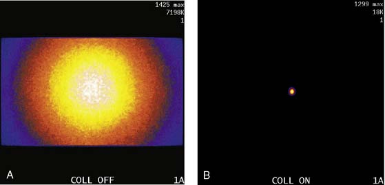
The third source of degradation discussed in this chapter is the finite, distance-dependent spatial resolution of the imaging system. When imaging in air, the system spatial resolution consists of two independent sources of blurring.9 The first is the intrinsic resolution of the detector and electronic components of the camera head. The second is the spatially varying geometric acceptance of the photons through the holes of the collimator. The collimator is the “lens” of the gamma camera; however, unlike optical lenses that form images by bending the light photons, collimators work by stopping all but the few photons that can pass through their holes without being absorbed by the septa of the collimator (absorptive collimation). This is illustrated in Figure 6-5, which shows two images of a very small point source of 99mTc at the same location 10 cm from the detector face, first with no collimator and then with a low-energy high-resolution (LEHR) parallel-hole collimator on the camera head. The obvious need for the collimator is made clear by this figure, and so is the price paid for the use of the collimator in terms of loss in detection efficiency. Without the collimator, 7.2 million counts were collected in 1 minute. With the collimator, only 18,000 counts were collected in 1 minute, or 0.25% of that when the collimator was not on the system. The actual difference is greater because when the collimator was off, the count rate was near the maximum count rate of the system, so the recorded number of counts was depressed by resolving time count losses.9
As good as the image of the point source looks in Figure 6-5B compared to 6-5A, the ideal response would have been significantly better, since the point source was approximately only 1 mm in any dimension, and its bright representation in Figure 6-5B is larger than 10 mm across. The image resulting from imaging a point source of activity such as illustrated in Figure 6-5B is called a point spread function (PSF),9 and it portrays how a very small source of activity is blurred out during the course of imaging. Figure 6-6A illustrates plots through the center of Monte Carlo–simulated PSFs for an increasing distance of the point source in air from the face of a LEHR parallel-hole collimator. Notice how the PSF changes significantly in width and height as a function of distance. However, the area under the curves stays constant, consistent with no change in sensitivity with distance in air from the face of a parallel-hole collimator.
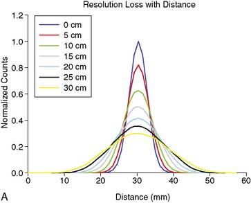
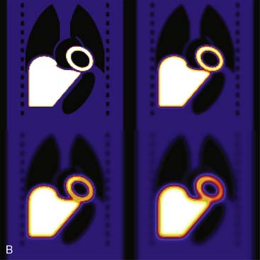
Figure 6-6B illustrates the impact of distance-dependent spatial resolution on one coronal slice through the MCAT phantom. As illustrated at the upper left in this figure, the concentrations of activity in the wall of the left ventricle (LV) and liver were the same, and that of the general tissue background was set to one-tenth that of the heart. All other organs had a concentration of activity of zero, as illustrated by the lungs, blood pool, and bones showing up as black. The slice at the upper right is that of the upper left blurred as if it were 10 cm from the face of a camera, as imaged with a LEHR collimator. The lower left slice is blurred as if acquired at 20 cm from the face of the collimator, and the lower right is 30 cm from the face. The FWHMs of the PSFs at these distances were 0.8 cm, 1.34 cm, and 1.88 cm. Notice how with increasing distance, the heart wall appears to become thicker and of apparently lower concentration relative to the liver. The apparent change in concentration is an illustration of the PVE or dependence of the apparent concentration of a structure on its size relative to the extent of blurring (FWHM).9 Note that the thickness of the wall in the slice varies due to the angulation of the heart relative to the coronal plane. Thus, the PVE causes the heart wall to appear as though it does not have a uniform concentration, when it actually had to begin with. Notice also that with increased distance, the liver and heart blur together to an increasing extent.
ESTIMATION OF PATIENT-SPECIFIC ATTENUATION MAPS
As illustrated in Figure 6-2, to accurately correct a given patient for the decrease in counts resulting from attenuation, it is necessary to know how the photons were attenuated when imaging that patient. That is, a patient-specific map of attenuation coefficients (μ), or attenuation map, is required. A number of methods exist for estimating such maps.3,4,6,7 In this chapter, we will discuss just those based on the idea of determining the attenuation of a beam of x-rays or gamma rays passing through the patient, which we will call transmission imaging. Transmission imaging consists of positioning a source of radiation (radionuclide or x-ray tube) on one side of the patient and a detector on the other side to measure the transmitted intensity. By taking the ratio of the transmitted intensity to the intensity without the patient present, the TF of Eq. 1 is determined. Because it is μ that we wish to estimate, Eq. 1 can be rearranged to solve for μ as follows:
where x is the distance traveled by the photon through the medium. In actuality, what one obtains on the right side of Eq. 3 is the sum of the attenuation coefficients that the photons travel through in going from the source to the detector, with each attenuation coefficient multiplied before summing by the length in pixels of that attenuation coefficient through which the beam passed. This is identical to the ideal case in emission imaging, where the counts one obtains in a pixel of an acquisition image are the result of the sum of the counts per pixel detected. Thus, just as the rows from the same level in emission images acquired around the patient can be used to reconstruct the emission image, rows from transmission images altered as per Eq. 3 can be used to reconstruct attenuation maps using FBP or some iterative algorithm. The question now is how one acquires the transmission information.
Basic Transmission Configurations
The basic transmission source and camera collimator configurations currently offered commercially are illustrated in Figure 6-7 for a 40-cm field of view (FOV) SPECT system imaging a 50-cm diameter patient. The first configuration illustrated in Figure 6-7A is that of a scanning line source.21 The camera head opposed to the line source is electronically windowed to store only the events detected in a narrow region opposed to the line source in the transmission image. This results in significant reduction in the amount of scattered transmission radiation from the source itself, imaged compared to having a stationary planar source opposite the camera. It also decreases (but does not eliminate) the cross-contamination from emission photons, because only the portion of the camera face where there is a high likelihood of a transmission photon being detected is used to form the transmission image. The emission images can also be electronically windowed to store counts only when the transmission source is not opposed to the location of the detected event. This simplifies the correction for down-scatter from a higher-energy transmission source to a lower-energy emission source window if different radionuclides are used or for self-correction if the same radionuclide is used for both emission and transmission imaging. This type of system is susceptible to problems in the mechanical motion of the line source and coordination of mechanical scanning with electronic scanning. Therefore, as part of one’s quality-control plan for attenuation compensation with such units, checks of the proper operation of the source scanning mechanism should be made frequently (daily) by performing a “blank” scan, which is a transmission scan with nothing, including the table, between the line source and camera head. One should also check individual patient transmission scans for signs of non-uniform motion in the axial (scanning) direction, truncation of the patient’s body within the FOV of the system, significant crosstalk from the emission-to-transmission source, and excessive attenuation of the transmission source by extra-large patients or weak sources.22 The merits of this configuration have made it the most widely available configuration for transmission imaging.
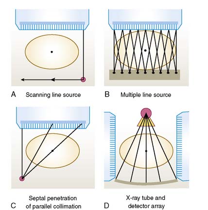
The second configuration, which is shown in Figure 6-7B, is that of the multiple line-source array.23 With this configuration, the transmission flux comes from a series of collimated line sources aligned parallel to the axis of rotation of the camera. The spacing and activity of the line sources are tailored to provide a greater flux near the center of the FOV, where the attenuation from the patient is greater. As the line sources decay, new line sources are inserted into the center of the array. The rest of the lines are moved outward and the weakest is removed. The transmission profiles result from the overlapping irradiation of the individual lines, which varies with the distance of the source from the detector. The multiple line-source array provides full irradiation across the FOV of the parallel-hole collimator employed for emission imaging, without the need for translation of the source. An advantage of the configuration is that no scanning motion of the sources is required. A disadvantage of this system is the amount of crosstalk between the emission and transmission photons. Thus, attenuation maps formed with this system when imaging 99mTc-labeled agents should be checked for apparent decreases in the attenuation coefficients (display intensity) in regions of significant 99mTc accumulation, such as the heart and liver. Also, the down-scatter of the transmission source to the 201Tl x-ray window makes the use of sequential or interleaved emission and transmission imaging favors. Another disadvantage is the high cost of replacing the line sources at short time intervals.
The first commercial transmission imaging system employed a line source at the focal distance of a fan-beam collimator.24 The major problem with using fan-beam collimation for estimation of attenuation maps is that of truncation. Truncation of attenuation profiles results in the estimated attenuation maps exhibiting the “cupping artifact,” or pile-up of information in the truncated region near its edge when the reconstruction is limited to reconstructing only the region within the FOV at every angle, or fully sampled region (FSR). If the reconstruction is not limited to the FSR, the area outside the FSR is distorted, and the inside is slightly reduced in value. Truncation can be eliminated, or at least dramatically reduced, by imaging with an asymmetric as opposed to a symmetric fan-beam collimator.25–28 The use of asymmetric collimation results in one side of the patient being truncated instead of both. By rotating the collimator and source 360 degrees around the patient, conjugate views will fill in the region truncated. If a point source with electronic collimator is employed instead of a line source, then a significant improvement in crosstalk can be obtained.29 The problem, however, is that fan-beam collimators acquire the emission profiles, which makes it difficult for physicians to use in cine-mode to check for attenuation artifacts when reading the patient studies. This difficulty is overcome by the third commercial method of transmission imaging currently being marketed, as illustrated in Figure 6-7C, by using photons from a medium-energy scanning point source to create an asymmetric fan-beam transmission projection through a parallel-hole collimator by penetrating the septa of the collimator.30 With this strategy, transmission imaging is performed sequentially after emission imaging to prevent transmission photons from contaminating the emission data. This lengthens the time the patient must remain motionless on the imaging table, thereby decreasing patient throughput and increasing the potential for patient motion. In particular, there is a change in motion of the heads between emission and subsequent transmission imaging, which can lead patients to momentarily relax, thinking the study is over, and thereby cause a misalignment between the emission data and attenuation map. Use of dual display in which the reconstructed emission slices are displayed in color “on top of” the reconstructed attenuation map displayed in grayscale, is recommended with this system to check for a possible misalignment.
High-resolution images from another modality can be imported and registered with the patient’s SPECT data.31,32 Of course, the task is made a lot simpler by acquiring the high-resolution slices while the patient is on the same imaging table.33 The inclusion of a computed tomography (CT) system on the SPECT gantry is the fourth transmission imaging option currently being offered commercially34 and is illustrated in Figure 6-7D. The use of a CT to estimate attenuation maps and provide anatomic correlation has essentially replaced the use of radionuclide-based transmission imaging in PET.35 CT overcomes the noise limitations of radionuclide transmission imaging through use of the x-ray tube and a separate block of detectors for x-ray imaging. However, the x-ray beam is made up of photons of many different energies. Thus appropriate care must be taken in scaling the attenuation map measured with this polychromatic photon beam to that of the energy of the emission radionuclide.36 Besides their use for attenuation maps, these images can also provide anatomic contexts for the emission distributions and compensation for the PVE.37 Because different detectors are employed, the CT and SPECT acquisitions are performed sequentially. Thus, as with the scanning medium-energy point source, care must be taken to assess the possibility of patient motion between the two, and imaging time is protracted.
There are two types of CT scanners in hybrid SPECT/CT. The first type is with a low-output x-ray tube and a slow gantry rotation cycle.34,38,39 A typical CT scan is taken with the x-ray tube current of 2.5 mA and the gantry rotation cycle of 23 seconds. It can be a single- or multiple-detector row CT scanner. It uses 13.6 seconds of data (little over half of a gantry rotation, due to fan-beam detector geometry) for reconstruction of a CT image. The CT image is not for diagnosis; rather, it is intended for attenuation correction of the SPECT data. The radiation dose of the slow CT is about 5 mGy, which is significantly less than that of CT when used for diagnostic imaging.39 Studies have demonstrated its effectiveness for this purpose.40 However, a recent study suggested caution when performing AC with this technology for evaluation of perfusion defects; the SPECT slices after AC might be compromised by misregistration between the attenuation map derived from the CT slices and the SPECT data.38 In this study, motion resulted in 42% of the 60 patients having moderate to severe misregistration of the heart between the CT and the SPECT data. Since most respiratory cycles are in the range of 4 to 6 seconds,41 the scan duration of 13.6 seconds for each CT image slice may not be slow enough to reduce reconstruction artifacts and subsequent misregistration. This is compounded by a possible change in respiration between emission and CT imaging, as well as a shifting in position of the patient. A recent study of using slow CT for respiratory gating suggested the gantry rotation cycle might have to be over 3 minutes to reduce the artifact caused by respiration.42 This is to ensure that there is one respiratory cycle of data taken at each CT projection angle.
The second type of CT scanner is diagnostic-quality CT, capable of producing thin slices of high spatial and temporal resolutions with a fast gantry rotation cycle of less than 0.6 seconds. The number of detector rows is 2, 6, 16, 40, or 64. The CT scanner can be potentially used for imaging the coronary arteries. However, the 64-detector row CT with 0.35 second or faster gantry rotation cycle produces the best image quality for the coronary artery, owing to its larger coverage and higher temporal resolution. The combination of CT for imaging coronary arteries and SPECT for evaluation of myocardial perfusion provides a noninvasive evaluation of the heart in both anatomy and function. Calcium scoring can also be obtained from this type of CT scanner to provide long-term risk assessment.43,44 Although the quality of CT is very good, it still poses problems in registration of the heart between CT and SPECT, because the CT image is taken in less than 1 second. Misregistration normally occurs when the CT image is taken at the end-inspiration phase, which is very different from the average respiration SPECT data of over several minutes. Recent development of “average CT” by averaging the CT images taken over one respiratory cycle may provide a solution.41,45 Average CT is promising in cardiac PET/CT46 and potentially useful for cardiac SPECT/CT. This approach uses a fast gantry rotation of less than 0.5 second to acquire CT images that are almost motion free in respiration, and averaging brings temporal resolution of the CT images to that of SPECT images. Acquisition of average CT data should be at least one respiratory cycle and can be carried out at a low tube current such as 10 mA and fast gantry rotation cycle of 0.5 seconds. The radiation dose of average CT is also about 5 mGy.41 Since the patient is scanned sequentially, re-registration of the CT and SPECT data manually is necessary if the patient moves between the CT and SPECT scans.46,47
ATTENUATION CORRECTION METHODS
Not only has the ability to estimate attenuation maps improved greatly, but so has the ability to perform correction of attenuation once the attenuation maps are estimated. In part, this is due to the tremendous changes in computing power available, with computers in the clinic now making computations practical that could only be performed as research exercises 10 years ago. It is also due to an improvement in the algorithms used for correction and the efficiency of their implementations. An example of this is the development of ordered subset or block iterative algorithms for use with the statistically based reconstruction methods discussed elsewhere.48–50 A number of algorithms have been developed for compensation of attenuation. The reader is referred to other reviews for more details and other algorithms.3, 5–7,51 In this review, we will focus on the group of methods that are replacing FBP.
Statistically Based Reconstruction Methods
The statistically based reconstruction algorithms start with a model for the noise in the emission data and then derive an estimate of the source distribution based on some statistical criterion. Many times they are named so that the first part of their name tells the statistical criterion that is to be optimized, and the second part of the name tells the mathematical algorithm employed to achieve optimization. For example, in MLEM,52,53 the statistical criterion is to determine the source distribution in the slices with the maximum likelihood (ML) of having resulted in the measured SPECT projection data, given that the noise fluctuations in the acquisitions follow the Poisson distribution. The expectation maximization algorithm is employed for finding this ML solution. The success of this method of reconstruction is reflected by its becoming the standard for comparison against other reconstruction methods.
Conceptually, the MLEM algorithm works by iteratively refining an initial guess as to the distribution of the counts in the slices until the distribution is found that has the greatest likelihood of having resulted in the measured SPECT acquisitions. The rule or algorithm followed can be summarized as51:
The algorithm starts on the bottom right hand side of Eq. 4 by mathematically emulating SPECT imaging of the current estimate (making projections from Slicesold). This is where the physics of imaging can come into play and is one of the major advantages of iterative methods over FBP reconstruction. One can include as much information as to how the estimated counts contribute to the acquired projections as one has the ability to mathematically model (and is willing to spend the computer time so doing) during each iteration. For example, given an aligned attenuation map for a slice, one could include attenuation by starting with the voxel on the side opposite the projection being created, and multiplying its value by the TF for passing through one-half the voxel distance of an attenuator of the given attenuation coefficient in the attenuation map. The value of half the pixel dimension is usually used as an approximation for the self-attenuation of the activity in the voxel. One would then move to the next voxel along the direction of projection, and add its value after correction for self-attenuation to the current projection sum attenuated by passing through the entire thickness of the voxel. One would then continue this process until having passed through all voxels along the path of projection. The result would be the discrete approximation to the calculation of the line integral through the emission estimate, with each voxel location corrected for attenuation. Similarly, one can include modeling of scatter-dependent and distance-dependent spatial resolution. It is our experience that the better one does at accurately mathematically modeling the imaging of the patient, the better the resulting image quality will be. Of course, without clever approximations, such modeling can be quite time-consuming, even with today’s computers. Thus implementations of MLEM will vary, depending on the extent to which the physics is modeled and the approximations are employed in implementation.
The second step in the MLEM algorithm, as shown by the division on the right side of Eq. 4, is to divide the estimated projection values into the values actually measured. The ratio of the two indicates whether the voxel values along the given path of projection are too large (ratio less than 1), just right (ratio of 1), or too small (ratio larger than 1). These ratios are then backprojected as indicated in Eq. 4 to create an update matrix. That is, the ratios are combined for each slice voxel according to the probability they contributed to the projections from which the ratios were formed. This update matrix is then normalized by dividing by the backprojection of 1.0s to account for some ratios contributing more than others to the update matrix, based on the physics of imaging. The normalized update matrix is then multiplied voxel-by-voxel times the old estimate of the slice values to create the new estimate. This step is typically repeated until a set number of iterations has been performed. Ordered subset expectation maximization (OSEM)48,49 and block iterative methods50 accelerate reconstruction by forming and applying the update matrix from subsets of the projection set that are selected in an ordered fashion. The result is a reduction in the number of iterations by a factor approximately equal to the number of subsets used.54 If fewer than four angles spaced as far apart as possible are used in forming subsets, then a loss in image quality with OSEM can result.55
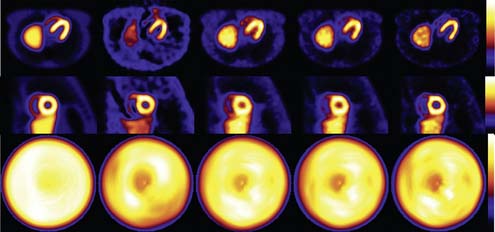
Figure 6-8 shows a comparison of the transverse slices, short-axis slices, and polar maps for reconstructions of simulations of the MCAT phantom.11 In the first column on the right are image slices and the polar map for the case FBP reconstruction over 360 degrees of Monte Carlo–simulated acquisition images created as imaged by a LEHR collimator but without inclusion of attenuation, scatter, or additional noise. Because no noise was added to the high-count Monte Carlo simulation, no low-pass smoothing was included with reconstruction. These images thus represent the case of ideal attenuation and scatter correction. Notice that the counts at the apex of the LV in the transverse slice and in the apical region of the polar map are not uniform. The non-uniformity reflects the impact of the PVE on wall counts due to the inclusion of apical thinning in the MCAT source distribution. This shows that even with ideal attenuation and scatter correction, one should not expect to obtain uniform counts in the polar maps. The following columns show what happens when attenuation and scatter in addition to distance-dependent spatial resolution are included in the Monte Carlo–simulated projections. Additionally, a noise level equivalent to that seen clinically is simulated, thus requiring low-pass filtering of the reconstructed slices. In the first column of these (second column of images from the left) are shown the results for FBP reconstruction of projection data that include attenuation acquired over the 180 degrees centered on the heart. A two-dimensional pre-reconstruction Butterworth filter with an order of 5 and a cutoff frequency of 0.25 cycle/cm was used to suppress noise. Notice the significant count fall off as one moves basally (deeper into the patient) along the myocardial walls, especially for the inferior wall. Also notice the distortion in shape of the walls, especially near the base. The center column of images shows the result of one iteration of OSEM reconstruction that employed 15 subsets of 4 angles each and included AC as described in the proceeding paragraphs. Additionally, three-dimensional (3D) post-reconstruction Gaussian filtering was applied to reduce noise. Notice that the shape of the LV walls is improved with AC, and the decrease in counts inferiorly is replaced with an increase septally and inferiorly. This overcorrection is due to the presence of scattered photons in the projections, which add counts to the projection data such that the decrease due to attenuation is moderated. The correction of attenuation is usually based on correcting the losses of primary counts. When these losses are corrected and scatter has not been removed, an apparent overcorrection by attenuation correction occurs.
SCATTER CORRECTION METHODS
The best way to reduce the effect of scatter would be to improve the energy resolution of the imaging systems by using an alternative to NaI(T1) scintillation detection.9 For such a system, the Gaussian function representing the distribution of primary photons with energy in Figure 6-4 would shrink to a single vertical line, with the result that very few scattered photons would be included in the energy window.
The Compton window subtraction (CWS) method of Jaszczak and colleagues represents a classic example of an energy domain scatter-estimation method that is still in clinical use.56 In the CWS method, a second energy window placed below the photopeak window (see Fig. 6-4) is used to record an image that consists of scattered photons. This image is multiplied by a scaling factor, k, and then subtracted from the acquired image to yield a scatter-corrected image. This method assumes that (1) the spatial distribution of the scatter within the Compton scatter window is the same as that within the photopeak window, and (2) once determined from a calibration study, a single scaling factor (k) holds for all applications on a given system. That the distribution of scatter between the two windows is different can be seen by noting that the average angle of scattering, and hence degree of blurring, changes with energy. The difference in the distribution of scatter with energy can be minimized by making the scatter window smaller and placing it just below the photopeak window. With this arrangement, one obtains the two energy window (TEW) variant of the triple energy window (also TEW) scatter-correction method of Ogawa and colleagues57 as applied to 99mTc. When down-scatter (scattered photons from a higher-energy emission) is present, a third small window is added above the photopeak, and scatter is estimated as the area under the trapezoid between the two narrow windows on either side of the photopeak.58 In this way, TEW can be used with radionuclides such as 201Tl, which emit photons of multiple energies, or for scatter correction when imaging multiple radionuclides.
In RBSC, a unique scatter PSF is estimated for each location in the patient, using a patient-specific attenuation map and the underlying principles of scattering interactions. This scatter PSF is then included in the projection and backprojection operations of iterative reconstruction. With RBSC methods, compensation is achieved in effect by mapping scattered photons back to their point of origin instead of trying to determine a separate estimate of the scatter contribution to the projections.59 All of the photons are used in RBSC, and it has been argued that there should be less noise increase than with the other category of compensations.59,60 The first RBSC method for SPECT was the inverse Monte Carlo method.61 This algorithm provided compensation for scatter, attenuation, and system resolution by using a Monte Carlo simulation to estimate the PSFs. Because obtaining a “noise-free” estimate of the PSFs with Monte Carlo methods is extremely time-consuming, a number of approximate methods have been investigated, which provide excellent compensation in computationally acceptable reconstruction times.59,60 More recently, methods of vastly speeding up Monte Carlo simulation have been developed such that for 99mTc, fully 3D reconstruction can be obtained in approximately 30 minutes on a personal computer.62
Comparison of the images of the center and second from the right columns in Figure 6-8 shows an example of the application of one of the RBSC methods to correct the simulated projection images from the MCAT phantom. OSEM reconstruction with the same reconstruction and smoothing parameters was used for both the images seen in both columns. Notice that with the addition of scatter correction, the cardiac blood-pool region is seen with higher contrast with respect to the walls, and the overcorrection in the septal and inferior walls is moderated somewhat. Also, there is slightly better separation between the liver and inferior wall. However, further separation between the two requires an improvement in reconstructed spatial resolution.
SPATIAL RESOLUTION COMPENSATION METHODS
If the PSF is the same for every point in the patient, then knowledge of it can be used to calculate restoration filters or mathematic filters that attempt to balance deblurring the slices with controlling noise.63 However, the in-air PSF for nuclear medicine cameras increases in width with distance away from the face of collimators, as illustrated in Figure 6-6. Therefore, the accuracy of correction methods that assume it is unchanging is limited. The frequency-distance relationship (FDR) can be used to separate out the signal in sinograms (matrix containing all the projections to be used in reconstructing a slice arranged according to the angle they were acquired at) according to the distance at which the signal originated relative to the collimator face.64 Once the distance is known, then a model for how spatial resolution changes as a function of distance from the face can be used to create restoration filters that account for the distance dependence of the PSF.65,66 Application of the FDR to restoration filtering SPECT acquisitions has advantages in terms of computational load and being linear. It also has several disadvantages.67 For example, it is limited as to how much resolution recovery can be obtained without excessive amplification of noise; modeling the distance-dependent spatial resolution directly in the projection and backprojection steps of iterative reconstruction has been determined to significantly improve the detection accuracy of tumors over use of it in observer studies using simulated images.68
Another method to correct for the distance-dependent camera response is the incorporation of a blurring model into iterative reconstruction.69–71 Returning to Eq. 4, the idea is as follows: When creating the estimate of projection data acquired from the current estimate of the source activity distribution, the values in that distribution are smoothed equivalent to how the camera blurs counts at that given distance before they are combined to form the projection. This is illustrated in Figure 6-6B, where the coronal plane is smoothed various amounts as a function of the distance to the collimator face. You can envision this happening in reconstruction by dividing the current 3D estimate of the source into a set of oblique planes perpendicular to the rays making it through the parallel-hole collimator. Each plane is then smoothed an increasing amount as the distance between them and the collimator face increases. Combining the smoothed planes with accounting for attenuation and scatter results in the estimated projection values, which are then compared to the actual acquired values by being divided into them. The question then arises as to how smoothing can lead to an improvement in resolution. The answer is that the actual source distribution was smoothed during the process of acquisition, just as we are now smoothing our estimate of the source distribution. When our estimated projections, with smoothing included, match the actual projection data we acquire, the estimated source distribution should match the actual source distribution imaged. Thus as we iterate, we sharpen our estimate of the source distribution until the smoothed version of its projections matches the data we acquired.
The problem with this method has been the immense increase in computational burden imposed when an iterative reconstruction algorithm includes such modeling in its transition matrix. Combined with OSEM, blurring incrementally with distance, using the method of Gaussian diffusion72 during projection and backprojection, can dramatically reduce the computational burden per iteration. With this method, correction for the system spatial resolution is incrementally changed with distance during projection and backprojection so that only a few voxels need to be combined at each distance from the face of the collimator. The increase in computational speed using this and similar algorithms is now such that reconstruction can be easily accomplished in clinically feasible times.
An illustration of the impact of including modeling of system spatial resolution in reconstruction is provided by a comparison of the images in the last two columns of Figure 6-8. The last column adds resolution compensation to compensation of attenuation and scatter, as illustrated in the next to last column. Notice the dramatic change in size of the blood-pool cavity, the thinning of the LV walls, and the improved separation from the liver. There is, however, a trade-off between gains in apparent image spatial resolution and increasing the noise content of the image. Thus by increasing the number of iterations and/or decreasing extent of post-reconstruction filtering, a further increase in apparent resolution at the expense of a further increase in the noise content of the images can be obtained.
EXAMPLE OBSERVER STUDIES ILLUSTRATING THE UTILITY OF COMPENSATION
Using the channelized-Hotelling numeric observer, Frey and colleagues showed with simulated cardiac studies that the best coronary artery disease (CAD) detection accuracy results when attenuation, scatter, and spatial resolution are included in iterative reconstruction.73 They determined an area under the receiver operating characteristic (ROC) curve, or AUC, of 0.90 for iterative reconstruction with solely AC, an AUC of 0.93 for iterative reconstruction with AC and spatial resolution compensation (RC), an AUC of 0.93 for AC and scatter correction (SC), and an AUC of 0.94 for combined AC, SC, and RC.
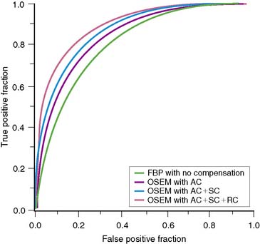
In a recent ROC comparison of detection accuracy for CAD of four different reconstruction strategies, using images from 100 patient studies read independently by seven physicians, Narayanan and colleagues determined that there was an additive improvement in detection accuracy as one progresses from FBP without additional compensation, to OSEM with AC, to OSEM with AC and SC, to OSEM with AC, SC, and Gaussian diffusion–based RC (Fig. 6-9).74 OSEM with AC, SC, and RC was determined to have a statistically larger AUC compared with FBP, or OSEM with solely correction for AC, hence improved diagnostic accuracy.
In the previous study, as is standard for comparisons of FBP and iterative reconstruction, only the stress slices were viewed by the physicians. When interpreting studies, clinically significant additional information is available to the physician. Pretorius and colleagues performed an ROC comparison of FBP and OSEM with AC, SC, and RC in which present when viewing the FBP studies were the short- and long-axis slices for both stress and rest, cines of the acquisition data for both stress and rest, a cine of selected gated cardiac slices, polar maps, and indication of whether the patient was male or female.75 Solely the stress short- and long-axis slices were made available to the observers for OSEM with combined correction. The inclusion of this additional information normally available clinically did increase the AUC for FBP from 0.81 for the previous study to 0.87 for this study. However, OSEM with combined correction still resulted in a statistically significant improvement in the detection accuracy of CAD, with an AUC of 0.90.
CONCLUSIONS
When carefully implemented and validated hardware and software are used to perform attenuation compensation, an improvement in the detection accuracy can be achieved clinically. When attenuation compensation is combined with compensation for scatter and distance-dependent spatial resolution, an ever greater improvement in detection accuracy can be expected to occur. To achieve these increases, it is necessary that the physician take time to become familiar with the appearance of these corrected images.76 Also, just as SPECT increased diagnostic accuracy over planar scintigraphy at the cost of increased demands on the performance of the imaging systems, so too the addition of attenuation compensation does increase diagnostic accuracy but at the price of needing to take more care with quality control. Finally, even though the degradation of SPECT images by attenuation, scatter, and the finite distance-dependent spatial resolution of the cameras employed in imaging is not debated, the extent to which these degradations can currently be routinely and robustly overcome in practice is still the subject of debate, exemplified in a pair of recent manuscripts.77,78
1. DuPuey D.J., Garcia E.V. Optimal specificity of thallium-201 SPECT through recognition of imaging artifacts. J Nucl Med. 1989;30:441.
2. Hendel R.C., Corbett J.R., Cullom S.J., et al. The value and practice of attenuation correction for myocardial perfusion SPECT imaging: A joint position statement from the American Society of Nuclear Cardiology and the Society of Nuclear Medicine. J Nucl Cardiol. 2002;9:135.
3. Bacharach S.L., Buvat I. Attenuation correction in cardiac positron emission tomography and single-photon emission computed tomography. J Nucl Cardiol. 1995;2:246.
4. King M.A., Tsui B.M.W., Pan T.S. Attenuation compensation for cardiac single-photon emission computed tomographic imaging: Part 1. Impact of attenuation and methods of estimating attenuation maps. J Nucl Cardiol. 1995;2:513.
5. King M.A., Tsui B.M.W., Pan T.S., et al. Attenuation compensation for cardiac single-photon emission computed tomographic imaging: Part 2. Attenuation compensation algorithms. J Nucl Cardiol. 1996;3:55.
6. Bailey D.L. Transmission scanning in emission tomography. Eur J Nucl Med. 1998;25:774.
7. Zaidi H., Hasegawa B.H. Determination of the attenuation map in emission tomography. J Nucl Med. 2003;44:291.
8. Attix F.H. Introduction to Radiological Physics and Radiation Dosimetry. New York: John Wiley & Sons, 1983.
9. Cherry S.A., Sorenson J.A., Phelps M.E. Physics in Nuclear Medicine, ed 3. Philadelphia: Saunders, 2003.
10. Eisner R.L., Tamas M., Cloninger K., et al. Normal SPECT thallium-201 bull’s-eye display: Gender differences. J Nucl Med. 1988;29:1901.
11. Pretorius P.H., King M., Tsui B.M., et al. A mathematical model of motion of the heart for use in generating source and attenuation maps for simulating emission imaging. Med Phys. 1999;26:2323.
12. Knesaurek K., King M.A., Glick S.J., et al. Investigation of causes of geometric distortion in 180 degrees and 360 degrees angular sampling in SPECT. J Nucl Med. 1989;30:1666.
13. Germano G., Chua T., Kiat H., et al. A quantitative phantom analysis of artifacts due to hepatic activity in technetium-99m myocardial perfusion SPECT studies. J Nucl Med. 1994;35:356.
14. Nuyts J., Dupont P., Van D.M., et al. A study of the liver-heart artifact in emission tomography. J Nucl Med. 1995;36:133.
15. Ljungberg M., Strand S.E. A Monte Carlo program for the simulation of scintillation camera characteristics. Comput Methods Programs Biomed. 1989;29:257.
16. Nuyts J., Stroobants S., DuPuey D.J., et al. Reducing loss of image quality because of the attenuation artifact in uncorrected PET whole-body images. J Nucl Med. 2002;43:1054.
17. Bai C., Kinahan P.E., Brasse D., et al. An analytic study of the effects of attenuation on tumor detection in whole-body PET oncology imaging. J Nucl Med. 2003;44:1855.
18. Bai C., Shao L. A study of the effects of attenuation correction on tumor detection in SPECT oncology. IEEE Nucl Sci Symp Conf Rec (2004). 2004;5:3113-3117.
19. de Vries D.J., King M.A. Window selection for dual photopeak window scatter correction in Tc-99m imaging. IEEE Trans Nucl Sci. 1994;41:2771.
20. Hademenos G.J., King M.A., Ljungberg M.H., et al. A scatter correction method for Tl-201 images: A Monte Carlo investigation. IEEE Trans Nucl Sci. 1993;40:1179.
21. Tan P., Bailey D.L., Meikle S.R., et al. A scanning line source for simultaneous emission and transmission measurements in SPECT. J Nucl Med. 1993;34:1752.
22. DePuey E.G., Garcia E.V., Borges-Neto S., et al. Imaging guidelines for transmission-emission tomographic systems to be used for attenuation correction. J Nucl Cardiol. 2001;8:G51.
23. Celler A., Sitek A., Stoub E., et al. Multiple line source array for SPECT transmission scans: Simulation, phantom and patient studies. J Nucl Med. 1998;39:2183.
24. Tung C.H., Gullberg G.T., Zeng G.L., et al. Nonuniform attenuation correction using simultaneous transmission and emission converging tomography. IEEE Trans Nucl Sci. 1991;39:1134.
25. Chang W., Loncaric S., Huang G., et al. Asymmetric fan transmission CT on SPECT systems. Phys Med Biol. 1995;40:913.
26. Gilland D.R., Jaszczak R.J., Greer K.L., et al. Transmission imaging for nonuniform attenuation correction using a three-headed SPECT camera. J Nucl Med. 1998;39:1105.
27. Hollinger E.F., Loncaric S., Yu D.C., et al. Using fast sequential asymmetric fanbeam transmission CT for attenuation correction of cardiac SPECT imaging. J Nucl Med. 1998;39:1335.
28. LaCroix K.J., Tsui B.M.W. Investigation of 90 degree dual-camera half-fanbeam collimation for myocardial SPECT imaging. IEEE Trans Nucl Sci. 1999;46:2085.
29. Beekman F.J., Kamphuis C., Hutton B.F., et al. Half-fanbeam collimators combined with scanning point sources for simultaneous emission-transmission imaging. J Nucl Med. 1998;39:1996.
30. Gagnon D., Tung C.H., Zeng L., Hawkins W.G. Design and early testing of a new medium-energy transmission device for attenuation correction in SPECT and PET. IEEE Nucl Sci Symp Conf Rec (1998). 1999;3:1349-1353.
31. Fleming J.S. A technique for using CT images in attenuation correction and quantification in SPECT. Nucl Med Commun. 1989;10:83.
32. Meyer C.R., Boes J.L., Kim B., et al. Demonstration of accuracy and clinical versatility of mutual information for automatic multimodality image fusion using affine and thin-plate spline warped geometric deformations. Med Image Anal. 1997;1:195.
33. Blankespoor S.C., Xu X., Kaiki K., et al. Attenuation correction of SPECT using x-ray CT on an emission-transmission CT system: myocardial perfusion assessment. IEEE Trans Nucl Sci. 1996;43:2263.
34. Bocher M., Balan A., Krausz Y., et al. Gamma camera-mounted anatomical x-ray tomography: Technology, system characteristics and first images. Eur J Nucl Med. 2000;27:619.
35. Kinahan P.E., Hasegawa B.H., Beyer T. X-ray-based attenuation correction for positron emission tomography/computed tomography scanners. Sem Nucl Med. 2003;33:166.
36. LaCroix K.J., Tsui B.M.W., Hasegawa B.H., et al. Investigation of the use of x-ray CT images for attenuation compensation in SPECT. IEEE Trans Nucl Sci. 1994;41:2793.
37. Da Silva A.J., Tang H.R., Wong K.H., et al. Absolute quantification of regional myocardial uptake of 99mTc-sestamibi with SPECT: Experimental validation in a porcine model. J Nucl Med. 2001;42:772.
38. Goetze S., Wahl R.L. Prevalence of misregistration between SPECT and CT for attenuation-corrected myocardial perfusion SPECT. J Nucl Cardiol. 2007;14:200.
39. Patton J.A., Turkington T.G. SPECT/CT Physical Principles and Attenuation Correction. J Nucl Med Technol. 2008;36:1.
40. Masood Y., Liu Y.H., Depuey G., Taillefer R., Araujo L.I., Allen S., Delbeke D., Anstett F., Peretz A., Zito M.J., et al. Clinical validation of SPECT attenuation correction using x-ray computed tomography-derived attenuation maps: multicenter clinical trial with angiographic correlation. J Nucl Cardiol. 2005;12:676.
41. Pan T., Mawlawi O., Luo D., Liu H.H., Chi P.C., Mar M.V., Gladish G., Truong M., Erasmus J.Jr, Liao Z., Macapinlac H.A. Attenuation correction of PET cardiac data with low-dose average CT in PET/CT. Med Phys. 2006;33:3931.
42. Lu J., Guerrero T.M., Munro P., Jeung A., Chi P.C., Balter P., Zhu X.R., Mohan R., Pan T. Four-dimensional cone beam CT with adaptive gantry rotation and adaptive data sampling. Med Phys. 2007;34:3520.
43. Berman D.S., Hachamovitch R., Shaw L.J., Friedman J.D., Hayes S.W., Thomson L.E., Fieno D.S., Germano G., Wong N.D., Kang X., Rozanski A. Roles of nuclear cardiology, cardiac computed tomography, and cardiac magnetic resonance: Noninvasive risk stratification and a conceptual framework for the selection of noninvasive imaging tests in patients with known or suspected coronary artery disease. J Nucl Med. 2006;47:1107.
44. Hecht H.S., Budoff M.J., Berman D.S., Ehrlich J., Rumberger J.A. Coronary artery calcium scanning: Clinical paradigms for cardiac risk assessment and treatment. Am Heart J. 2006;151:1139.
45. Pan T., Mawlawi O., Nehmeh S.A., Erdi Y.E., Luo D., Liu H.H., Castillo R., Mohan R., Liao Z., Macapinlac H.A. Attenuation correction of PET images with respiration-averaged CT images in PET/CT. J Nucl Med. 2005;46:1481.
46. Gould K.L., Pan T., Loghin C., Johnson N.P., Guha A., Sdringola S. Frequent diagnostic errors in cardiac PET/CT due to misregistration of CT attenuation and emission PET images: a definitive analysis of causes, consequences, and corrections. J Nucl Med. 2007;48:1112.
47. Goetze S., Brown T.L., Lavely W.C., Zhang Z., Bengel F.M. Attenuation correction in myocardial perfusion SPECT/CT: effects of misregistration and value of reregistration. J Nucl Med. 2007;48:1090.
48. Hudson H.M., Larkin R.S. Accelerated image reconstruction using ordered subsets of projection data. IEEE Trans Med Imaging. 1994;13:601.
49. Hutton B.F., Hudson H.M., Beekman F.J. A clinical perspective of accelerated statistical reconstruction. Eur J Nucl Med. 1997;24:797.
50. Byrne C.L. Block iterative methods for image reconstruction from projections. IEEE Trans Image Process. 1996;5:792.
51. Bruyant P.P. Analytic and iterative reconstruction algorithms in SPECT. J Nucl Med. 2002;43:1343.
52. Shepp L.A., Vardi Y. Maximum likelihood reconstruction for emission tomography. IEEE Trans Med Imaging. 1982;1:113.
53. Lange K., Carson R. EM reconstruction algorithms for emission and transmission tomography. J Comput Assist Tomogr. 1984;8:306.
54. Meikle S.R., Hutton B.F., Bailey D.L., et al. Accelerated EM reconstruction in total-body PET: Potential for improving tumour detectability. Phys Med Biol. 1994;39:1689.
55. Gifford H.C., King M.A., Narayanan M.V., et al. Effect of block iterative acceleration on Ga-67 tumor detection in thoracic SPECT. IEEE Trans Nucl Sci. 2002;49:50.
56. Jaszczak R.J., Greer K.L., Floyd C.E.Jr, et al. Improved SPECT quantification using compensation for scattered photons. J Nucl Med. 1984;25:893.
57. Ogawa K., Ichihara T., Kubo A. Accurate scatter correction in single photon emission CT. Ann Nucl Med Sci. 1994;7:145.
58. Ogawa K., Harata Y., Ichihara T., et al. A practical method for position-dependent Compton-scatter correction in single photon emission CT. IEEE Trans Med Imaging. 1991;10:408.
59. Kadrmas D.J., Frey E.C., Tsui B.M.W. Application of reconstruction-based scatter compensation to thallium-201 SPECT: Implementations for reduced reconstructed image noise. IEEE Trans Med Imaging. 1998;17:325.
60. Beekman F.J., Kamphuis C., Frey E.C. Scatter compensation methods in 3D iterative SPECT reconstruction: A simulation study. Phys Med Biol. 1997;42:1619.
61. Floyd C.E., Jaszczak R.J., Coleman R.E. Inverse Monte Carlo: A unified reconstruction algorithm. IEEE Trans Nucl Sci. 1985;32:785.
62. Beekman F.J., de Jong H.W.A.M., van Geloven S. Efficient fully 3-D iterative SPECT reconstruction with Monte Carlo-based scatter compensation. IEEE Trans Med Imaging. 2002;21:867.
63. King M.A., Schwinger R.B., Doherty P.W., et al. Two-dimensional filtering of SPECT images using the Metz and Wiener filters. J Nucl Med. 1984;25:1234.
64. Edholm P.R., Lewitt R.M., Lindholm B. Novel properties of the Fourier decomposition of the sinogram. Proc Soc Photo Opt Instrum Eng. 1986;671:8.
65. Lewitt R.M., Edholm P.R., Xia W. Fourier method of correction of depth-dependent collimator blurring. Proc Soc Photo Opt Instrum Eng. 1989;1092:232.
66. Glick S.J., Penney B.C., King M.A., et al. Noniterative compensation for the distance-dependent detector response and photon attenuation in SPECT imaging. IEEE Trans Med Imaging. 1994;13:363.
67. Kohli V., King M.A., Glick S.J., et al. Comparison of frequency-distance relationship and Gaussian-diffusion-based methods of compensation for distance-dependent spatial resolution in SPECT imaging. Phys Med Biol. 1998;43:1025.
68. Gifford H.C., King M.A., Wells R.G., et al. LROC analysis of detector-response compensation in SPECT. IEEE Trans Med Imaging. 2000;19:463.
69. Floyd C.E.Jr, Jaszczak R.J., Manglos S.H., et al. Compensation for collimator divergence in SPECT using inverse Monte Carlo reconstruction. IEEE Trans Med Imaging. 1987;35:784.
70. Tsui B.M.W., Hu H.B., Gilland D.R., et al. Implementation of simultaneous attenuation and detector response correction in SPECT. IEEE Trans Nucl Sci. 1987;35:778.
71. Zeng G.L., Gullberg G.T., Tsui B.M.W., et al. Three-dimensional iterative reconstruction algorithms with attenuation and geometric point response correction. IEEE Trans Med Imaging. 1990;38:693.
72. McCarthy A.W., Miller M.I. Maximum likelihood SPECT in clinical computation times using mesh-connected parallel computers. IEEE Trans Med Imaging. 1991;10:426.
73. Frey E.C., Gilland K.L., Tsui B.M.W. Application of task-based measures of image quality to optimization and evaluation of three-dimensional reconstruction-based compensation methods in myocardial perfusion SPECT. IEEE Trans Med Imaging. 2002;21:1040.
74. Narayanan M.V., King M.A., Pretorius P.H., et al. Human-observer ROC evaluation of attenuation, scatter, and resolution compensation strategies for Tc-99m myocardial perfusion imaging. J Nucl Med. 2003;44:1725.
75. Pretorius P.H., King M.A., Dahlberg S.T., et al. Detection accuracy of coronary artery disease of FBP with all the clinically available imaging information compared to iterative reconstruction with combined compensation for imaging degradations. J Nucl Cardiol. 2005;12:284.
76. Corbett J.R., Ficaro E.P. Attenuation corrected cardiac perfusion SPECT. Curr Opin Cardiol. 2000;15:330.
77. Garcia E.V. SPECT attenuation correction: an essential tool to realize nuclear cardiology’s manifest destiny. J Nucl Cardiol. 2007;14:16.
78. Germano G., Slomka P.J., Berman D.S. Attenuation correction in cardiac SPECT: the boy who cried wolf? J Nucl Cardiol. 2007;14:25.
[/level-membership-for-internal-medicine-category][not-level-membership-for-internal-medicine-category]
Chapter 6 Attenuation/Scatter/Resolution Correction
Physics Aspects
INTRODUCTION
A number of factors can cause artifacts in cardiac single-photon emission computed tomography (SPECT) imaging.1 Among these are the attenuation and scattering of the photons in the patient’s tissues and the finite and distance-dependent spatial resolution SPECT systems. A significant amount of research and development has gone into perfecting clinically robust compensation strategies for these. The present status of clinical trials has led the American Society of Nuclear Cardiology and the Society of Nuclear Medicine to jointly develop and publish a position statement on attenuation correction (AC), which concluded “that the adjunctive technique of attenuation correction has become a method for which the weight of evidence and opinion is in favor of its usefulness.”2 To achieve an improvement in diagnostic accuracy with AC, it is required for physicians to modify their “approach to image interpretation accounting for the effects of these methods on the resultant images,”2 and “use hardware and software that have undergone clinical validation and include appropriate quality-control tools (see Chapter 7).”2
It is our belief this recognition of the utility of AC will be followed by that of the need for also correcting for scatter and distance-dependent spatial resolution. Our position is that the more completely the physics of imaging is correctly included in reconstruction, the more accurate will be the diagnosis from the reconstructed slices. Thus, the goals of this chapter are to (1) provide an introduction to the physics of imaging and how this can be incorporated into reconstruction and (2) illustrate that when this is done, diagnostic accuracy can be improved. Other related reviews on this have been published by Bacharach and Buvat,3 King and colleagues,4,5 Bailey,6 and Zaidi and Hasegawa.7
IMPACT OF ATTENUATION, SCATTER, AND RESOLUTION ON CARDIAC SINGLE-PHOTON EMISSION COMPUTED TOMOGRAPHY (See Chapter 7)
Interactions and Exponential Attenuation
For a photon—whether gamma ray from technetium (99mTc) or x-ray subsequent to the decay of thallium (201Tl)—to become part of a cardiac image, it must first escape the body (see photon A in Fig. 6-1). The chances of this occurring are reduced in proportion to the likelihood that it will interact in the patient’s body before it can escape. At the photon energies of interest in nuclear cardiology, the major interactions in tissues are Compton scattering and photoelectric absorption.8,9 In Compton scattering, a photon interacts with an electron that is loosely bound compared to the photon’s energy. The result of this interaction is the ejection of the electron from the atom and the creation of a new photon having a lower energy and different direction (see photons B and C in Fig. 6-1). The probability of interaction per unit path length (characterized by the linear attenuation coefficient for Compton scattering) depends on the tissue density and number of electrons per gram and decreases slowly with increasing photon energy. In photoelectric absorption, the photon imparts all of its energy to an electron, which is then ejected from the atom. The ejected photoelectron carries a kinetic energy that is equal to the energy of the incident photon minus the binding energy with which it was held to the atom. No scattered photon is emitted in the photoelectric interaction (see photon D in Fig. 6-1). However, characteristic radiation will likely be emitted when the electrons of the atom rearrange to fill the vacancy left by the photoelectron. The linear attenuation coefficient for photoelectric absorption increases as the cube of the atomic number of the atom, depends on tissue density, and decreases as the inverse cube of the photon energy.
where μ is the linear attenuation coefficient (sum of all the coefficients for individual interactions) and x is the thickness of the attenuator the photons pass through. If the attenuator is made up of a number of materials of various compositions, then the product μx in Eq. 1 is replaced by a sum of the attenuation coefficient for each material times the thickness of the material the transmitted photons pass through (path length the photons travel in the material). As a result of the differences in attenuation coefficient with type of tissue, the TF will vary with the materials traversed, even if the total patient thickness between the site of the emission and the camera is the same. Thus, one needs to have patient-specific information on the spatial distribution of attenuation coefficients (an attenuation map) to calculate the attenuation, which decreases the probability of photon detection.
Attenuation Artifacts (See Chapter 6)
The change in TF with direction of the photons and between different locations in the patient results in a variation in attenuation. This can be visualized in planar images as, for example, breast shadows and decreased counts in the presence of an elevated diaphragm. In SPECT slices, these artificial shadows are difficult to recognize; however, there is a pattern of altered relative counts consistent with the influence of attenuation in the mean bull’s eye polar maps of patients with a low likelihood of CAD. Eisner and colleagues reported decreased relative counts in the anterior wall of 201Tl polar maps for females due to breast attenuation, and a relative decrease in the inferior wall of males, which may be due to diaphragmatic attenuation.10 The problem is that the location, extent, and severity of these reduced-count regions vary from patient to patient as a function of their anatomy. Thus, the variation in the pattern of apparent localization in disease-free patients is increased, resulting in more false-positive results (lower specificity) at any given level of true-positive results (sensitivity).
The types of changes in the reconstructed activity distributions when attenuation is present are illustrated in Figure 6-2. The top row of this figure shows what can be expected in the simple case of an elliptically shaped uniform-activity distribution without and with the presence of attenuation caused by a uniform attenuation distribution within the object. Note that attenuation causes a scaling of the reconstructed activity distribution such that there is a decrease by more than a factor of 2 at the outside, and a further decrease as one moves toward the center or most attenuated portion of the distribution. Hence an extended object that has a uniform distribution to begin with would have a loss in uniformity dependent on the relative depths of locations within it. The middle row of the figure shows the more complex case of a uniform source distribution that is attenuated by a non-uniform attenuation distribution simulating that of a cross-section through a female patient. This attenuation distribution and subsequent source and attenuator distributions the employed in the figures of this chapter were obtained from the mathematic cardiac-torso (MCAT) digital anthropomorphic phantom.11 Notice that because the lungs have an attenuation coefficient approximately one-third that of soft tissue, there is now less attenuation within them than would have occurred had the entire cross-section consisted of soft tissues. Thus with attenuation, there appears to be a higher concentration of activity within them than the surrounding soft tissue, when actually the concentration was uniform. Notice also the sharp transition in apparent concentration of activity between the medial boundary of the lung and the heart region. The heart lateral wall is attenuated significantly more than the lung next to it. This explains why AC correction is very sensitive to having the correct registration between emission imaging and attenuation maps. A small movement can cause a big difference in the correction applied. The bottom row shows the even more complex case of both non-uniform source and attenuation distributions from the MCAT phantom simulating that of 99mTc-sestamibi imaging. At the far left, in the absence of attenuation, the distribution of activity within the heart wall is uniform; however, when attenuation is included, a non-uniform distribution results, with the apex and lateral wall being brighter than the deeper lateral wall. Notice also that with attenuation present, there is now a mild change in the size and shape of the heart, as well as a significant distortion of the liver. With attenuation, there now is activity reconstructed as being outside the body. Such geometric distortion is greater for 180-degree reconstruction (as performed for these slices) than 360-degree reconstruction, owing to the greater inconsistencies in the emission profiles in the absence of their averaging by combining conjugate views.12 The positive and negative tails from hot sources, which result from the incomplete cancellation of the inconsistent data in the emission profiles, can also lead to significant distortions in cardiac wall counts when there is significant extracardiac localization, such as with hepatic uptake. Germano and colleagues showed in phantom studies that an apparent reduction in counts occurs with the presence of a “hot” liver in the slices with the heart.13 Nuyts and colleagues14 observed that use of 360 degrees as opposed to 180 degrees with filtered backprojection (FBP) reconstruction reduced the magnitude of the artifact. The artifact was further reduced by use of attenuation compensation with maximum-likelihood expectation-maximization (MLEM) reconstruction.
The artifactual decrease in apparent activity within the heart walls due to nearby extracardiac activity is further illustrated in the short-axis slices and circumferential count profiles at the top of Figure 6-3 for 180-degree reconstruction of Monte Carlo simulations15 of the MCAT phantom.11 The top set of slices are with the liver uptake simulated as the same as that of the background. The next lower set of three slices shows the artifactual decrease in the inferior wall caused by the alteration of the liver activity to be the same as that of the heart. This alteration is illustrated graphically in the plots of the maximum count circumferential count to the right. There, one sees the typical pattern of a decrease in activity in the inferior versus the anterior wall due to the greater depth of the inferior wall, but this difference is dramatically accentuated by the increase in liver activity. This alteration in the apparent distribution of activity within the slices can be understood by the theory of the impact of attenuation on positron emission tomography (PET) and SPECT slices developed by Nuyts et al.,16 Bai et al.,17 and Bai and Shao.18 By this theory, attenuation causes a scaling of the counts at a given position, as illustrated in Figure 6-2, and a shifting of the local counts due to the attenuation of the other activity within the slice. It is this shifting that creates a negative bias that is the cause of the artifactual decrease in the inferior wall of the heart.
That AC, when included within iterative reconstruction, can correct this artifactual decrease as illustrated in the middle set of three short-axis slices at the left in Figure 6-3, and in the corresponding circumferential profile at the right. Notice that with AC, the wall now becomes fairly uniform in uptake. Notice also that the liver now becomes more intense than the heart, even though they were simulated as having the same concentration of activity. The reason for the apparent difference is the partial volume effect (PVE),9 which causes structures smaller in any dimension than two to three times the full-width-at-half-maximum (FWHM) measure of the system spatial resolution to be blurred such that their apparent activity is less than the actual value.
Broad Beam Attenuation and Scatter
Equation 1 is accurate only (1) for a beam of photons with the same energy and (2) under the “good geometry condition” that, as soon as a photon undergoes any interaction, is no longer counted as a member of the beam.8,9 Attenuation coefficients measured subject to these conditions are the “good-geometry” attenuation coefficients. Compton scattered photons, even though they are reduced in energy, are not necessarily excluded from being counted, owing to the finite width of the energy windows used because of the limited ability to distinguish different energy photons (finite energy resolution) of the cameras (Fig. 6-4). In fact, the ratio of scattered photons included in the energy window to primary photons in the energy window (scatter fraction) is typically 0.34 for 99mTc19 and 0.95 for 201Tl20 for cardiac SPECT. Thus, Eq. 1 has to be modified to match the “broad beam” attenuation, which actually occurs in emission imaging by the inclusion of the buildup factor B, which is dependent on both μ and x. The result is8,9:
When scatter is not removed from the emission profiles before reconstruction, or its presence is incorporated into the reconstruction process itself, an overcorrection will occur. This is illustrated by the three sets of short-axis slices and the circumferential profiles at the bottom of Figure 6-3. As discussed previously, the top row of these slices illustrates how successful AC included within MLEM reconstruction can be at correcting the artifactual change in apparent uptake of the inferior wall of the row of slices just above it. However, the success of AC returning this slice to an apparent uniform concentration of activity within the walls is due in part to just primary photons being present. When the scattered photons acquired within the photopeak of the simulated acquisition are included, the short-axis slices next to the bottom are obtained. Notice how scatter has caused the inferior wall to now appear brighter than the anterior wall, which is the opposite of the effect of attenuation. The presence of scatter has also decreased wall contrast compared to the heart chamber region and visually decreased the separation of the heart from the liver. The bottom row of short-axis slices shows this is due to the non-uniform presence of scatter being concentrated closer to the liver. The circumferential profiles at the bottom right in the figure show that quantitatively, scatter has added approximately 30% more counts to the heart wall and that the inferior wall was increased the most.
Finite and Distance-Dependent Spatial Resolution
The third source of degradation discussed in this chapter is the finite, distance-dependent spatial resolution of the imaging system. When imaging in air, the system spatial resolution consists of two independent sources of blurring.9 The first is the intrinsic resolution of the detector and electronic components of the camera head. The second is the spatially varying geometric acceptance of the photons through the holes of the collimator. The collimator is the “lens” of the gamma camera; however, unlike optical lenses that form images by bending the light photons, collimators work by stopping all but the few photons that can pass through their holes without being absorbed by the septa of the collimator (absorptive collimation). This is illustrated in Figure 6-5, which shows two images of a very small point source of 99mTc at the same location 10 cm from the detector face, first with no collimator and then with a low-energy high-resolution (LEHR) parallel-hole collimator on the camera head. The obvious need for the collimator is made clear by this figure, and so is the price paid for the use of the collimator in terms of loss in detection efficiency. Without the collimator, 7.2 million counts were collected in 1 minute. With the collimator, only 18,000 counts were collected in 1 minute, or 0.25% of that when the collimator was not on the system. The actual difference is greater because when the collimator was off, the count rate was near the maximum count rate of the system, so the recorded number of counts was depressed by resolving time count losses.9
As good as the image of the point source looks in Figure 6-5B compared to 6-5A, the ideal response would have been significantly better, since the point source was approximately only 1 mm in any dimension, and its bright representation in Figure 6-5B is larger than 10 mm across. The image resulting from imaging a point source of activity such as illustrated in Figure 6-5B is called a point spread function (PSF),9 and it portrays how a very small source of activity is blurred out during the course of imaging. Figure 6-6A illustrates plots through the center of Monte Carlo–simulated PSFs for an increasing distance of the point source in air from the face of a LEHR parallel-hole collimator. Notice how the PSF changes significantly in width and height as a function of distance. However, the area under the curves stays constant, consistent with no change in sensitivity with distance in air from the face of a parallel-hole collimator.
Figure 6-6B illustrates the impact of distance-dependent spatial resolution on one coronal slice through the MCAT phantom. As illustrated at the upper left in this figure, the concentrations of activity in the wall of the left ventricle (LV) and liver were the same, and that of the general tissue background was set to one-tenth that of the heart. All other organs had a concentration of activity of zero, as illustrated by the lungs, blood pool, and bones showing up as black. The slice at the upper right is that of the upper left blurred as if it were 10 cm from the face of a camera, as imaged with a LEHR collimator. The lower left slice is blurred as if acquired at 20 cm from the face of the collimator, and the lower right is 30 cm from the face. The FWHMs of the PSFs at these distances were 0.8 cm, 1.34 cm, and 1.88 cm. Notice how with increasing distance, the heart wall appears to become thicker and of apparently lower concentration relative to the liver. The apparent change in concentration is an illustration of the PVE or dependence of the apparent concentration of a structure on its size relative to the extent of blurring (FWHM).9 Note that the thickness of the wall in the slice varies due to the angulation of the heart relative to the coronal plane. Thus, the PVE causes the heart wall to appear as though it does not have a uniform concentration, when it actually had to begin with. Notice also that with increased distance, the liver and heart blur together to an increasing extent.
