Assessment of visual function
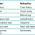
3.1 Differential diagnosis information from other assessments
3.3 Near visual acuity (and near vision adequacy)
3.4 Central visual field screening
3.5 Central visual field analysis
3.6 Peripheral suprathreshold visual field screening
3.7 Central 10 degree visual field analysis
3.8 Visual field assessment for drivers
3.9 Gross visual field screening
3.1 Differential diagnosis information from other assessments
3.2 Distance visual acuity
3.2.1 When should distance visual acuity be measured?
There are three principal measures of VA:
• Unaided VA, often called vision.
• Habitual VA, with the patient’s own spectacles.
• Optimal VA, with the best refractive correction, i.e. after subjective refraction.
VA after objective refraction is also often recorded. Either vision and/or habitual VA should be measured immediately after the case history for legal reasons, to document the VA level prior to your examination. Habitual and optimal distance VA are routine measurements. Measuring distance unaided VA (vision) is optional, and should be measured with patients who:
• have lost/broken their spectacles so that you cannot measure habitual VA;
• do not wear spectacles for some distance viewing tasks (this information must therefore be obtained in the case history);
• require the information for a report;
• wear their spectacles all the time for distance and yet you suspect they may not need to (does the young low hyperope need to wear the spectacles for distance tasks?)
3.2.2 LogMAR versus Snellen
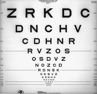
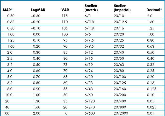
LogMAR visual acuity (VA) charts (Figure 3.1) use the design principles suggested by Bailey and Lovie, including 0.1 logMAR progression of letter size from −0.3 to 1.0 logMAR (equivalent to 6/3 to 6/60 or 20/10 to 20/200), five letters per line, letters of similar legibility and per-letter scoring.1 Snellen charts were devised by the German ophthalmologist Hermann Snellen in 1862 and have been widely used ever since. There is not a standard Snellen chart and the letter size sequences, number of letters and/or numbers, varieties of letters, etc., vary from manufacturer to manufacturer. They typically contain one letter at a VA level of 6/60 (20/200; 0.1 logMAR) and increasing number of letters at smaller letter sizes with a typical bottom line of about 6/5 or 20/15 (~ −0.1 logMAR).
The majority of Snellen charts have only one 6/60 or 20/200 letter, two 6/36 or 20/125 letters and three 6/24 or 20/80 letters. LogMAR charts typically have five letters on each of these lines and additional lines of letters at 6/30 or 20/100 (0.70 logMAR) and 6/48 or 20/160 (0.90 logMAR). Most logMAR charts have a ‘bottom line’ of −0.3 logMAR (6/3 or 20/10), whereas many Snellen charts have a bottom line of 6/5 or 20/15 and thus provide truncated data given that the average visual acuity of a young adult is about 6/4 (Table 3.1).2
Table 3.1
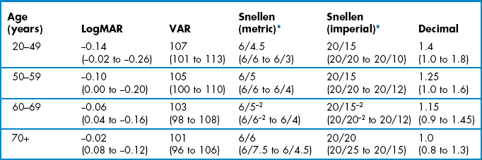
Normal age-matched visual acuity data for various notations.2 The average is shown with 95% confidence limits in brackets
LogMAR charts are widely recognised as providing the most reliable and discriminative VA measurements and are standard for clinical research or clinical trials of ophthalmic devices or drugs.3,4 Visual acuity measurements using a logMAR chart have been shown to be twice as repeatable as those from a Snellen chart and over three times more sensitive to inter-ocular differences in VA and therefore substantially more sensitive to amblyopic changes for example.3,5 The Bailey–Lovie or ETDRS charts are the most commonly used logMAR charts for adults and the Glasgow Acuity Cards (commercially available as the Keeler logMAR crowded charts) have been designed specifically for children.4,5
3.2.3 Procedure
 See online video 3.1.
1. Ensure the chart is at the appropriate distance and is calibrated correctly.
2. Leave the room lights on and illuminate the chart. The luminance of the chart should be between 80 and 320 cd/m2. Seat the patient comfortably with an unobstructed view of the test chart. You should sit in front and to one side of the patient in order to monitor facial expressions and reactions.
3. If you are going to measure both vision and habitual VA, measure vision first to avoid memorisation. To measure vision, ask the patient to remove any spectacles. To measure habitual visual acuity, ask the patient to put their distance vision spectacles on.
4. Measure the visual acuity of the ‘poorer’ eye first, if a poorer eye is known from previous records or from the case history (to avoid a patient memorising the letters seen with the better eye and giving a false visual acuity with the poorer eye. Note that this can be avoided with computer-based charts by randomising the letters prior to measurement). Otherwise, measure VA in the right eye first.
5. Explain what measurement you are about to take. This can be as simple as ‘Now we shall find out what you can see in the distance’.
6. Instruct the patient: ‘Please cover up your left/right eye with the palm of your hand/this occluder’. If using the patient’s hand, make sure that the palm is being used as otherwise the patient may be able to peek through their fingers. Some clinicians prefer to hold the occluder over the patient’s eye themselves to ensure it is properly occluded.
7. Ask the patient: ‘Please read the smallest line that you can see on the chart’ or similar.
8. Continually monitor the patient’s facial expressions and head position. Do not permit the patient to screw their eyes up or look around the occluder or through their fingers.
9. Once the patient has reached what they believe are the smallest letters they can see, they should be pushed to determine whether they can see any more. Use prompts such as ‘Can you see any letters on the next line?’ or ‘Have a guess. It doesn’t matter if you get any wrong’. Some patients are more cautious than others and only indicate those letters that they can see easily and clearly. Unless you push patients to guess, you could obtain different VA results depending on how cautious your patient is. Ideally, you should stop pushing patients to read more if they make four or more mistakes on a line of five letters.6
10. If the patient cannot see the largest letters on the chart, ask them to move closer to the letter until two or three lines can be seen (or use a printed panel chart at a reduced distance). The distance at which this occurs should be noted. This is a more accurate assessment than determining the position that the patient can ‘count fingers’.7 If the patient cannot see the letters even at the closest test distance, use the following test sequence. Stop at the level at which the patient can accurately respond.
(a) Hand movements (HM) @ Y cm: The patient can see a hand moving from a certain distance. Some computerised VA tests can provide accurate measurements down to the hand movements level and these should be used when available.7
(b) Light projection (Lproj.): The patient can report which direction light is coming from when you hold a penlight about 50 cm away. Ask the patient to point to the light and note the areas of the field in which the patient has light perception.
(c) Light perception (LP): The patient can see the light but not where it is coming from. If they cannot see light, the vision is recorded as no light perception or NLP.
3.2.4 Alternative procedures to assess VA in children
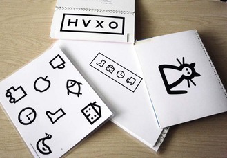
Amblyopia can be missed if single letters are used rather than a letter chart because of the lack of contour interaction. Ideally logMAR-based charts with contour bars at the end of lines, such as the logMAR crowded charts, should be used when measuring VA in children (Figure 3.2).8 The logMAR crowded charts have been shown to be over three times more sensitive to inter-ocular differences in VA than single letter Snellen charts and therefore substantially more sensitive to amblyopic changes.5 Crowded and standard and logMAR charts can even be used in children who do not know their letters by providing them with a key card that includes a selection of the letters from the chart. You then point to a letter on the chart and ask the child to identify the letter on their key card. For children that are unable to use a key card, charts are now available in logMAR format that include pictures rather than letters (Figure 3.2), such as the Kay crowded picture test, which has been shown to provide comparable results to the logMAR crowded charts.9
3.2.6 Recording for logMAR and Snellen charts
VA measurements can be scored in logMAR notation, using the visual acuity rating (VAR) score or converting scores to an equivalent Snellen value. Computer-based systems will typically convert VA values for you. LogMAR or VAR could be used on your own record cards. However, equivalent Snellen values should generally be provided when writing referral letters and reports, as Snellen notation is universally understood, whereas logMAR is not at present. In all cases, it is preferable to score using a by-letter system rather than measuring the lowest line at which the majority of letters were correctly read as it provides more repeatable and discriminative measurements.10 Comparisons of various logMAR scores with Snellen and other recording notations are shown in Table 3.2.
Table 3.2
Distance visual acuity conversion table
MAR, minimum angle of resolution; VAR, visual acuity rating.
The fact that logMAR VAs better than 6/6 or 20/20 are negative is counterintuitive. The VAR score provides a simpler method for scoring logMAR charts. VAR = 100 − 50 logMAR. Therefore 0.00 logMAR = 100 VAR and each letter has a score of 1. For example if a patient reads all the letters down to the 100 row and gets one letter wrong on this row, their score is 99, two letters wrong 98, etc. If they read all of the letters on the 100 row and one letter on the row below, their score is 101, two letters on the line below 102, etc. A disadvantage of the VAR score is that it suggests that 100 (6/6) is normal VA, which is far from true for many patients with healthy eyes.2
The Snellen fraction is defined as:
Test Distance/Distance at which the letters subtend 5 min of arc.
Test distance can be provided in metres (typical 6m) or feet (typically 20 feet).
Snellen VA can be labelled in either decimal or conventional Snellen notation (see Table 3.2 for comparison).
Vision or visual acuity is recorded as the smallest line in which the majority of the letters are seen, irrespective of subjective blur. Errors are recorded by appending a minus one, two or three to the Snellen fraction or decimal notation. If additional letters are seen on the following line, the Snellen fraction or decimal notation can be appended by a plus (usually up to no more than 3). If the patient could not see the 6/60 letter at 6 m, but could at 2 m, record 2/60. Similarly if the patient could not see the 20/200 letter at 20 feet, but could see the 20/120 letter at 5 feet, record 5/120.
Vision or ‘VA s Rx’ or VAsc or Vsc all mean visual acuity measured without a correction.
VAs are recorded for the right eye (RE or OD), left eye (LE or OS) and binocular (BE or OU).
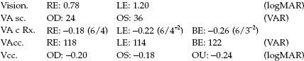
This last example is given in decimal format, which is commonly used in parts of Europe. It should not be confused with logMAR.
3.2.7 Interpretation
Any deviation from normal age-matched results, as shown in Table 3.1, should be noted. Note that the average VA for patients less than 50 is about −0.14 logMAR (6/4.5, 20/15) and that 6/6 or 20/20 represents reduced VA for the vast majority of patients. 6/6 or 20/20 only becomes the average VA for patients over 70 years of age with healthy eyes. You must also check whether there has been any change in VA from the previous examination. In patients with normal or near normal VA, a significant change in VA is more than 0.1 logMAR or one line.5,11 Also note any inter-ocular asymmetry of a line or more, or a binocular result that is worse than the monocular response.5
By comparing vision and optimal VA or habitual and optimal VA and using the one line of VA is equivalent to −0.25DS rule, an estimate of the mean spherical correction can be gained (section 4.1.5). If this estimate is widely different from the actual subjective refraction result, an error may be suspected and the subjective (and/or spectacle power) rechecked.
3.2.8 Most common errors
1. Allowing cautious patients to decide their acuity (i.e. not pushing them to guess).
2. Permitting the patient to screw their eyes up and improve their VA.
3. Permitting the patient to look around the occluder or through their fingers and view binocularly when measuring monocular VA.
4. Not recording the result immediately and guessing the result at the end of the examination.
5. Forgetting that patients could have VA better than your bottom line (of typically 6/5 or 20/15 with some Snellen charts).
3.3 Near visual acuity (and near vision adequacy)
3.3.1 Comparison of different near vision charts
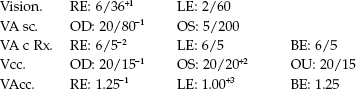
Near vision cards typically present sentences or paragraphs of words rather than isolated letters and can incorporate examples of near vision tasks such as sheet music, technical drawings and telephone directories (Figure 3.3). They are also now available on e-tablet and e-phones. There are five main types of notations used to measure near VA: logMAR, N-point, M-scale, equivalent Snellen, and Jaeger. LogMAR near charts have all the advantages of distance logMAR charts (section 3.2.2) and should be used whenever an accurate, non-truncated measurement of near VA is needed and particularly when distance VA and near VA may differ, such as with multifocal implants/contact lenses and patients with subcapsular cataract. Some near logMAR charts use isolated letters rather than words, but word charts are preferred, particularly in patients with conditions such as age-related macular degeneration as it relates better to reading performance and is typically worse than near letter VA.12 N-point uses the Times New Roman font and is the standard test in the UK and Australia. It is based on the ‘point size’ used by printers and word processing packages on modern computers, in which 1 point = 1/72 inch (~0.353 mm). This can be a useful aid when indicating to a patient the level of vision that would be provided for computer use by new lenses. N8 is approximately equal to 1.0 M and this eight times conversion holds for all print sizes. M-units are widely used in North America and indicate the distance in metres at which the height of a lower case ‘x’ subtends 5 minutes of arc. A 1.0 M letter ‘x’ is therefore 1.45 mm high. Equivalent Snellen notation is a confusing notation, especially when near VAs are not measured at the standard 16′: What does 20/20 near VA at 8′ mean? In addition, near vision adequacy should indicate what patients can see at their own near working distance, not an arbitrary standard of 16′ (working distances for reading in patients with normal vision range from 10′ to 20′13). Cards using Jaeger notation should not be used as there is no standardisation of what J1 or J5, etc., means and different charts can give totally different sizes of print with the same J-value.
3.3.2 Procedure: logMAR near VA and M or N-notation near vision adequacy
 See online video 3.2.
1. Sit in front and to one side of the patient in order to monitor facial expressions and reactions.
2. Measurements should be made in similar lighting conditions to those the patient uses at home. Ask if the patient uses an anglepoise or goose-neck light at home, and if they do, use additional light for your near VA measurements.
3. Instruct the patient to place the near vision card (or e-tablet, e-phone or e-book reader) at their normal near working distance. Measure and record this distance.
4. Measure the near VA of the ‘poorer’ eye first, if a poorer eye is known from previous records or from the case history. Otherwise, measure the right eye first. Use an occluder or the patient’s palm of their hand to cover the other eye. If using the patient’s hand, make sure that the palm is being used as otherwise the patient may be able to peek through their fingers.
5. Explain to the patient what measurement you are about to take. This may be a simple: ‘Now we shall find out what you can see at close distances’.
6. Instruct the patient to read the smallest paragraph they can.
7. Unless the patient can see the smallest print, push them to determine whether they can see anymore. Prompts such as ‘Try and make out some of the words in the smaller paragraph’ may be useful. Some patients are more cautious than others and only indicate those letters that they can see easily and clearly. Unless you push patients to guess, you could therefore obtain different near VA results depending on how cautious your patient is.
3.3.3 Adaptation for older patients
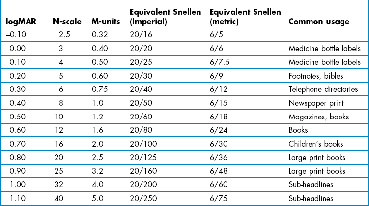
You should have asked the patient whether they use additional lighting, such as an anglepoise or goose-neck light, to read in their home. If they do not and you subsequently find they cannot easily read N5 (or 0.4 M) at the end of the reading addition part of the refraction, they should be encouraged to obtain additional light for near tasks in their home. It is very useful to demonstrate how helpful such additional light can be. The main objective of people with vision impairment is to be able to read and a majority can be successfully helped in primary eye care using high reading additions, simple magnifiers and additional lighting.14 Note that although near VA levels can be associated with a range of near tasks (Table 3.3), the poorer near VAs are threshold measurements (measurements of N5, 0.4 M and 20/20 may be truncated and not thresholds as discussed earlier) so that patients would not be able to read print of that size comfortably for any length of time. For example, to allow somebody to read newspaper print comfortably requires a near VA better than N8 or 1.0 M which is the typical size of newspaper print (Table 3.3) as a ‘reading reserve’ of 2 : 1 is needed and a near VA of N4 or 0.5 M.15
3.3.4 Recording
Note the working distance and then record the smallest paragraph size seen by the right and left eyes and binocularly. For approximate equivalents to other notations see Table 3.3. Some clinicians do not note the working distance unless it is different from the ‘norm’. However, even patients with good vision present a wide range of normal working distances (22 cm to 50 cm for reading,13 and further away for computer use), and as stated earlier a reading acuity is meaningless without a working distance. It can also be useful to record the working distance(s) used to determine near VA with the patient’s own spectacles to allow a comparison with the one used to determine the reading add. This can also be useful for comparison if patients return to your practice dissatisfied with the near vision in any new spectacles. These cases are often due to problems with working distance determination rather than an incorrect refraction.
3.3.5 Interpretation
When determining a reading addition, do not assume you have the correct add just because a patient can see the smallest text on your near chart such as N5, 0.4 M or 20/20. At 40 cm 0.4 M is equivalent to about 20/20 or 6/6 distance VA and N5 is equivalent to 6/9 or 20/30. Therefore, a patient could have reduced distance VA and still read N5, 0.4 M or 20/20 at near. Apart from this truncation effect, near VA can be expected to be similar to distance VA in most cases provided that the eye is accommodating normally or that the reading addition is correct. Notable exceptions include patients with multifocal intra-ocular lenses (IOLs) or wearing multifocal contact lenses or patients with posterior sub-capsular cataract. Patients with some eye disorders, such as amblyopia, age-related macular degeneration (ARMD) and macular oedema, can have significantly worse reading VA than distance VA and isolated-letter near VA.12
3.4 Central visual field screening
Perimetry enables the assessment of visual function throughout the visual field, the detection and analysis of damage along the visual pathway, and the monitoring of disease progression. Central visual field analysis using standard automated perimetry (SAP) can be a lengthy procedure and quicker and simpler techniques can be used for screening the central visual field. Central visual field screening should not be performed on patients with minimal risk factors (such as patients over 40 years of age without other risk factors, high myopes) due to the problems of false positive results when testing healthy patients (section 1.2).16 For example, the most commonly used screening programme for Frequency Doubling Perimetry is the N-30-5. The −5 in the programme title indicates that there is a 5% chance of a positive test being from a patient with a normal visual field, so that specificity is set at 95%. With a POAG prevalence of about 2%; out of 1000 patients, 20 would have POAG, but 980 would be healthy and 5% of them (49) would have a positive test result (49 false positives, ~72% of those with a positive result). Central visual field screening can be considered for patients who are asymptomatic with minor risk factors, such as patients with normal looking discs and intra-ocular pressures (IOP) but who have a primary family history of glaucoma, or who over 75 years, or over 30 years of age and black (African Caribbean, African American) where the prevalence of POAG is higher and false positives less of an issue (section 1.2).16 This is particularly true when positive tests are repeated. For patients exhibiting significant risk factors for glaucoma (abnormal appearing discs, high IOP), neurological disease, certain types of retinal disease or symptomatic patients, it is more appropriate to perform a central visual field analysis rather than use a screening technique.
3.4.1 Comparison of tests
The speed and accuracy of contemporary fast threshold estimation strategies have made several of the traditional screening techniques somewhat redundant. Fast thresholding strategies can produce an estimation of visual field sensitivity in a time (2.5–4 minutes per eye) similar to single stimulus, suprathreshold screeners. All of the fast central field analysis techniques have the advantage over suprathreshold screening techniques in that they are better able to detect early visual field defects, and can give an idea of defect depth and area. They have the disadvantage of taking longer than some suprathreshold techniques. They are similar in sensitivity and specificity for glaucoma as frequency doubling perimetry, but much better at detecting other types of visual field defect.17,18 When compared to techniques for full central field analysis they are quicker but less precise and with worse test-retest characteristics.19 The Humphrey Field Analyser (HFA) II, SITAFast (Swedish Interactive Thresholding Strategy), Central 24-2 tests 58 locations over the central 25° in a 6° grid pattern that straddles the horizontal and vertical mid-lines, i.e. targets are located 3° either side of the mid-lines. In addition there are targets located on the nasal field between 25° and 30°. The SITAFast, 24-2 programme rarely takes more than 3.5 minutes in a normal patient, and can be as quick as 2.5 minutes. Most modern perimeters have similar fast thresholding central visual field programmes.
3.4.2 Procedure
1. Explain the test and the reasons for performing the assessment to the patient.
2. When performing visual field screening pupils should be 3 mm or greater, whenever possible. It is considered acceptable to perform visual field testing whilst a pupil is dilating, provided the pupil is at least 3 mm at the start of the test. Note the position of the upper lid (i.e. possible blepharoptosis or dermatochalasis) and consider taping if it is obstructing the field of view.
3. Reduce ambient illumination and turn on the instrument.
4. For most visual field screeners: Contact lens wearers should perform the visual field test in their lenses. This is particularly useful for aphakes and high ametropes. Full aperture trial case lenses should otherwise always be used. Reduced aperture lenses and masked cylindrical lenses (i.e. those with opaque masks running along the direction of the axis) can result in visual field artefacts. Similarly bifocal and progressive addition glasses and those with small frames should be avoided. Best sphere should be used for any cylinder less than 1.50 D. If the cylinder is greater than 1.50 D then place the appropriate spherical lens in the back cell of the lens holder and the cylindrical lens in the cell immediately in front of the sphere. You should use a translucent occluder if the patient has latent nystagmus.
5. Seat the patient at the instrument and adjust the height of the instrument to ensure patient comfort. Over-extension of the neck and a bent back with hunched shoulders and neck should both be avoided.
6. Select ‘Central 24-2’ and then subsequently select ‘Change Parameters’ and ‘Test Strategy’ to ensure ‘SITAFast’ is used.
7. Select the eye to be tested first, and unless otherwise indicated select ‘Right’.
8. Enter the patient ID. Let the patient adapt to the bowl luminance while entering the data. This is a very important but frequently overlooked procedure, as it ensures a consistent level of retinal adaptation over the duration of the test. Enter as much patient data as possible but always include patient name using the surname first, date of birth (this is often formatted as month-day-year) and patient file number if appropriate. It is often useful to enter the prescription lenses used and pupil size. It is also possible to enter a diagnostic code, VA, IOP and cup-to-disc ratio.
9. Occlude the left eye and give the patient the response button.
10. Place the patient’s head in the headrest. Explain the test to the patient: ‘I want you to keep looking at the yellow light in the middle of the bowl. When you see a light flashing off to the side of the yellow light, please press this button. There will be times during the test when you will not be able to see any lights flashing and this is normal. Remember to keep looking at the yellow light in the middle of the bowl all the time’.
11. Align the patient using the video eye monitor.
12. Ensure that the vertex distance of the trial lens is adjusted appropriately and the trial lens is centred in front of the eye.
13. Select ‘Demo’ for a naive patient. Repeat until you are happy that the patient understands the procedure.
15. Some models will have a Gaze Monitoring feature. Once initialised, select ‘Start’.
16. Monitor fixation, check that the patient’s forehead has remained touching the rest and encourage the patient throughout the test. Use phrases such as ‘you are doing well’, ‘over half way now’, ‘keep looking straight ahead…that’s good’ or ‘you’ve nearly finished’. Do not leave the patient unattended.
17. When the test is completed, store the result on disk then select ‘Test Other Eye’. Occlude the patient’s right eye and align the left eye with the appropriate correction having been placed in the lens holder.
18. When the left eye is completed, store the results on disk and print the results if required.
3.4.3 Recording
If no test locations are highlighted on the Total and Pattern Deviation probability plots then record ‘SITA-Fast: WNL (within normal limits) R and L’. If there is a field defect, repeat the test, print and store both fields of both eyes and attach to the record card. SITA-Standard (or equivalent) could be used instead of SITA-Fast for the repeated field. The single field analysis of the repeated field should accompany any referral to the secondary eye care system. The single field analysis printout illustrates the data as an interpolated greyscale, raw data in decibels, and Total and Pattern deviation plots. It also summarises the field using the Glaucoma Hemifield Test, Global Indices, Reliability Indices, and Gaze Tracking plots (section 3.5.4).
3.4.4 Interpretation
These are interpreted in exactly the same way as the strategies for full central field analysis (section 3.5.4). It is important to be aware of the possible causes of artefact in cases where it would appear that a new defect has been detected, particularly in a patient with no previous experience of visual field screening or no history of field loss. A new defect is not a defect until it is repeated, ‘if in doubt always repeat’. The effect of learning and fatigue can be dramatic.20 Note that when the Glaucoma Hemifield Test classifies the field as having a ‘general reduction of sensitivity’, the Mean Defect/Deviation is abnormal and/or the Total Deviation probability plot shows a majority of test locations as being outside of normal limits, care should be taken when interpreting the results. There is usually an obvious clinical reason, with the most likely association being with cataracts or small pupils.
3.4.5 Most common errors
1. Using an inappropriate spectacle or lens type.
2. Poorly aligning the patient.
3. Providing poor patient instruction: It is worth investing time to ensure that the naïve patient understands what is expected of them. If necessary, repeat the test until you are satisfied that the patient has performed adequately.
3.5 Central visual field analysis
The most commonly used perimeter and programmes for central visual field analysis is the Humphrey Field Analyser (HFA) SAP programmes 30-2 and 24-2. The 30-2 programme tests 76 locations over the central 30° in a 6° grid pattern that straddles the horizontal and vertical mid-lines, i.e. targets are located 3° either side of the mid-lines.21 Equivalent programmes can be found on most perimeters. The 24-2 programme examines the central 25°, with the addition of more peripheral targets in the nasal step region, and consequently testing time is reduced by up to 20% compared to the 30-2 strategy. It is often used in follow-up assessments and to lessen the likelihood of any fatigue effect. Analysis of the central visual field should be performed on all patients with:
• Significant risk factors for glaucoma (compare with section 3.4) including, but not limited to, combinations of IOP >21 mmHg, old age, family history, narrow angles, vertical elongation of the optic nerve head, notching of the neural rim tissue of the optic nerve head, disc haemorrhage, nerve fibre layer defect, exfoliative syndrome, pigment dispersion, optic nerve head asymmetry.
• Abnormal screening test (e.g. positive screening test, confrontation or Amsler).
• Symptoms consistent with neurological disease (for example, headache including migraine, dizziness, tingling of limbs) or neuro-ophthalmic disease.
• Symptoms consistent with central field loss, e.g. non-refractive reduced vision, positive scotoma, scintillating scotoma.
In addition threshold fields are always required when monitoring a known defect, and they should always be included in protocols for the management of glaucoma.
3.5.1 Comparison of tests
The instrument should be capable of monitoring fixation, providing full threshold fields in less than 8 minutes, providing reliability indices and analysing the results. A rapid threshold estimation algorithm, such as the HFA’s SITAStandard or the Octopus Dynamic Strategy is recommended. These strategies take approximately 7 to 9 minutes per eye, without compromising the accuracy or repeatability of the result.22,23 The use of faster, less repeatable, thresholding strategies (e.g. HFA SITAFast and Octopus TOPs; section 3.4) may be considered as an alternative for some patients with a demonstrated history of fatigue. There has been discussion that SITA should not be used in patients suspected of conditions other than glaucoma as they are optimised specifically for glaucoma. However, clinically the advantage of the reduced test time makes such a compromise worthy of consideration, and no evidence has been presented that suggests a reduction in diagnostic capability for non-glaucomatous defects.
3.5.2 Procedure
The procedure for central visual field analysis is the same as that for central visual field screening (section 3.4.2) except that:
• At the ‘Main Menu’ select ‘Central 30-2’ (or ‘Central 24-2’).
• Select ‘Change Parameters’, followed by ‘Test Strategy’ and ensure ‘SITAStandard’ is selected. If a full threshold strategy is considered appropriate, select ‘Full Threshold’.
• If false negative catch trials are noted, advise the patient to rest by keeping the response button pressed down which will pause the test.
• If false positive catch trials are noted, pause the test by keeping the response button pressed down and re-instruct the patient.
3.5.3 Recording
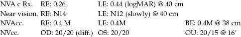
If no test locations are highlighted on the Total and Pattern Deviation probability plots then record ‘SITA-Standard (30-2): WNL (Within Normal Limits) R and L’. Print the fields for both eyes and attach to the record card. If a new defect has been detected, particularly in a patient with no previous experience of perimetry or no history of field loss, then repeat the field measurement. Confirmation of visual field abnormalities is essential for distinguishing reproducible visual field loss from long-term variability (section 1.2). The single field analysis printout illustrates the data as an interpolated greyscale, raw data in decibels, and Total and Pattern deviation plots (Figure 3.4). It also summarises the field using the Glaucoma Hemifield Test, Global Indices, Reliability Indices, and Gaze Tracking plots. When monitoring glaucoma, the Guided Progression Analysis (GPA), which is based upon the Early Manifest Glaucoma Trial, is designed to identify true glaucoma progression.24
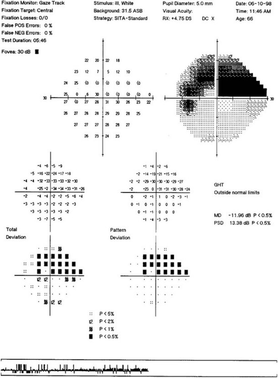
Fig. 3.4 The printout includes the sensitivity level for each point in decibels; an interpolated grey scale display; the total deviation in decibels and probability of each point being normal in a non-interpolated grey scale; the pattern deviation in decibels and probability of each point being normal in a non-interpolated grey scale; the glaucoma hemifield test; the gaze track plot; and global indices.
3.5.4 Interpretation
Reliability indices
The reliability indices consist of the following (for a review see Lalle)25:
Fixation losses: These are assessed by presenting suprathreshold targets in the blind spot (Heijl-Krakau technique). They are flagged if more than 20% occur, however this has been found to be too stringent and 30% is a more appropriate cut-off.26 If fixation losses are flagged, only discard the field if you feel that the patient was struggling to fixate, or if false negatives are also flagged.
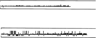
The HFAII also employs gaze-tracking throughout the test, displayed as a bar chart on the monitor and the printout (Figure 3.5). Upward deflections indicate eye movements and downward deflections are recorded when the position of the eye cannot be determined or there is a blink.
False positives: These errors indicate a ‘trigger happy’ patient who is responding to the sound of the perimeter when no target is presented. They should be less than 20%. Intervene immediately if false positives start to appear during the test and re-instruct the patient. If false positives are greater than 20%, the result should be discarded and the field repeated. For a repeat field, the test speed could be reduced.
False negatives: These errors accumulate when a patient fails to respond to a suprathreshold target at a given location; these are associated with fatigue and/or inattention. They should also be less than 20%. If you notice false negatives accumulating, particularly toward the end of an examination, give the patient a rest. This will often ensure that the false negative score does not reach significance. If the false negative rate does not improve, despite a rest, it can be better to continue on another day.
Single field analysis
The single field analysis (Figure 3.4) includes: the sensitivity level for each point in decibels; an interpolated grey scale display; the total deviation in decibels and probability of each point being normal in a non-interpolated grey scale; the pattern deviation in decibels and probability of each point being normal in a non-interpolated grey-scale and the glaucoma hemifield analysis. The Octopus and Oculus perimeters also include a defect curve.
• Total deviation (TD) compares the result to an age-matched normal population and states the probability of each point being abnormal on a point-by-point basis.
• Pattern deviation (PD) compares the result to an age-matched normal population corrected for the overall level of sensitivity for the individual. The probability of any point varying from this level is stated on a point-by-point basis. This enhances the ability to observe mappable scotomata within a generalised depression, which may be induced by small pupils or poor media.
• If there are no abnormal points on the TD and PD plots, then the patient can be considered as having a normal field.
• A generalised depression will be most easily appreciated by looking for a majority of abnormal points on the TD probability chart. Clusters of two or more non-edge points together on the PD chart (p < 0.05) should be considered suspicious. An isolated point within the central 10° (p < 0.05) should also be considered suspicious. If a cluster of abnormal points exists it should be interpreted with respect to its underlying anatomical correlate and subsequent clinical significance. Many artefacts show large jumps in sensitivity, from −1 to −28 dB for example.
• The glaucoma hemifield test analyses the relative symmetry of five pre-defined areas in the superior and inferior field, as well as judging the overall level of sensitivity compared to age-matched normal values. The visual field is then classified as being ‘within normal limits’, ‘outside normal limits’, ‘borderline’, ‘abnormally high sensitivity’, or to have a ‘general reduction of sensitivity’. Note that some other visual defects are not picked up by the glaucoma hemifield test, so it should not be relied upon to interpret all visual field losses. The defect curve ranks the test locations from most to least sensitive and plots relative to the 5% and 95% confidence interval for normal visual fields.
The global indices
The global indices are data reduction statistics designed to describe specific characteristics of the glaucomatous visual field.27 In summary:
• Mean deviation (MD) is the mean difference in decibels between the ‘normal’ expected hill of vision and the patient’s hill of vision. If the deviation is significantly outside the norms, a p-value will be given. It is useful to monitor the overall change in the visual field (Figure 3.6a).
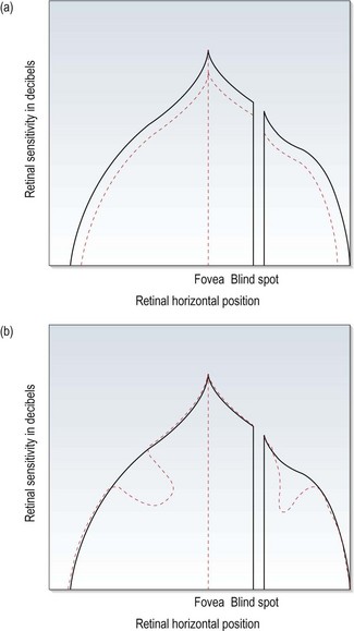
Fig. 3.6 The hill of vision, showing changes that would produce (a) a significant mean defect (MD) and (b) a significant pattern standard deviation (PSD).
• Pattern standard deviation (PSD) is a measure of the degree to which the shape of the patient’s field deviates from age-matched normal. A low PSD indicates a smooth hill of vision, while a high PSD indicates an irregular hill. PSD characterises localised changes in the visual field (Figure 3.6b). The value is expressed in decibels and any value of 2dB or greater will have a p-value next to it indicating the significance of the deviation. Note that it gets better as the field defect advances to more severe stages, as the field becomes more uniform once again.
• Short-term fluctuation (SF) is a measure of the intra-test variance. It has proven to be of little clinical value.
• Corrected pattern standard deviation (CPSD) is PSD corrected for the SF. These latter two indices are no longer provided on SITA fields.
The probability of the global indices being normal is stated on the printout.
Visual field progression
Change in the visual field of a single patient over time is best appreciated using the Overview printout. Caution is recommended when considering change in the visual field due to the high level of inter-test variability, particularly when a defect is present.28 The mantra should be ‘if in doubt always repeat’. If a glaucomatous defect is being followed, the Guided Progression Analysis (GPA) can be considered (see online figure 3.4vi). This is a refinement of the original Glaucoma Change Probability analysis and was developed for the Early Manifest Glaucoma Trial. GPA uses the pattern deviation database rather than the total deviation database, and is therefore more robust to the effects of cataract and reduced pupil size. The analysis uses estimates of the inherent variability within glaucomatous visual fields. This is combined with the Early Manifest Glaucoma Trial criterion of three significantly deteriorating points repeated over three examinations. A minimum of two baseline and one follow-up examination are required. Each exam is then compared to baseline and to the two prior visual fields. Abnormal points are highlighted, as are those that progress on two or three consecutive examinations.
3.6 Peripheral suprathreshold visual field screening
3.6.1 Comparison of tests
The recommended approach to peripheral field testing is to first record a fast threshold central test (see section 3.4) followed by a peripheral suprathreshold screening programme that tests between 30 and 60 degrees. Similar programmes can be found on most modern bowl perimeters. Alternate methods would include a full field suprathreshold screening programme or combining a fast threshold central test with a fast threshold peripheral test. It should be noted that there has been no comparison of these different approaches.
Virtually all visual field defects, including those due to chiasmal or post-chiasmal lesions, are reflected within the central 30° visual field.29 This is simply due to the anatomy of the visual pathway. There is a systematic bias towards representation of the central visual field, with over 80% of the visual pathway dedicated to processing the central 30° of vision.30
3.6.2 Procedure
The example used is the Humphrey Field Analyser, Three-zone, Peripheral 60.
1. Following completion of the 30-2 programme select ‘Screening’ test type from the ‘Main Menu’.
4. Select ‘Change Parameters’.
5. Select ‘Three Zone’ test strategy.
6. Select ‘Age Reference Level’ test mode.
7. Follow steps 7 to 18 of Section 3.4.2.
8. Print results as a merged file with the central 30 degree threshold result, if possible.
3.7 Central 10 degree visual field analysis
The most common assessment of central visual function is visual acuity measurement. However, this provides just one assessment of central vision and offers little help in differential diagnosis. In addition, some ocular abnormalities can produce little or no reduction in visual acuity, but can produce other changes to central vision, such as centrocaecal scotomas, metamorphopsia (distorted vision) and changes in colour vision. Although central visual field should be assessed in patients with suspect age related maculopathy, those taking certain medications such as hydroxychloroquine that are known to occasionally cause maculopathy and similar conditions, structural measures such as SD-OCT (section 7.11) can provide earlier diagnoses.31
3.7.1 Comparison of tests
Standard automated perimetry has been shown to be much more sensitive, specific, reliable and valid for detecting central visual field changes than Amsler charts.32,33 Standard Amsler charts are high contrast and even threshold adaptations of the chart (using cross-polarising filters) are poor at detecting scotomas smaller than 6°.32 Schuchard also found that more than half of the distortion reported in Amsler grids was at retinal locations that corresponded to the location of scotoma. Amsler charts rely heavily on subjective interpretation and may also be compromised by the ‘completion phenomena’, which perceptually fills small gaps in line stimuli.33
The Amsler Grid is an alternative to 10° central visual field analysis if a quick assessment of macular function is required and it is particularly useful in cases with metamorphopsia or visual distortion. Amsler charts have the advantage that they are portable, so can be used for home visits. The recording sheets can be used for home monitoring, although compliance has been shown to be poor and it is likely that the white-on-black Amsler charts are more sensitive to macular changes than the black-on-white recording sheets.34,35
3.7.2 Procedure for the Humphrey Field Analyser 10-2 programme
The same as central visual field analysis but replace programme 30-2 with programme 10-2 (Section 3.5.2).
3.7.3 Procedure for Amsler charts
1. Seat the patient comfortably in the examining chair with the appropriate near correction. As the working distance for the test is 30 cm, ideally a 3.25 D near add should be used for absolute presbyopes. However, the patient’s own spectacles are usually satisfactory given sufficient depth of focus. Use single vision glasses or trial lenses, but avoid multifocal lenses.
2. Position yourself so as to be able to occlude the non-viewing eye and measure the working distance. Get the patient to hold the chart at 30 cm.
3. Keep the room lights on. The method is qualitative and critical light levels are not essential; however, it is useful to be able to reproduce approximate ambient luminance levels.
4. Select the chart for testing:
(a) Chart 1: the standard chart used in every case. Consists of a 5 mm square, white grid with each square subtending approximately 1° from 30 cm, on a black background with a central, white fixation target.
(b) Chart 2: similar to chart 1 but with two diagonal white lines to assist steady fixation in patients with a central scotoma.
(c) Chart 3: similar to Chart 1 but with a red grid. It has been reported to be useful in the toxic amblyopias and optic neuritis, but is also capable of testing the malingerer when used in conjunction with red and green filters.
(d) Chart 4: consists of scattered white dots with a central, white fixation target. It appears no more sensitive than the standard chart for relative scotomas and cannot detect metamorphopsia.
(e) Chart 5: consists of white parallel lines only and a central, white fixation point. The chart can be rotated to change the orientation of the lines and is used to investigate metamorphopsia along specific meridians.
(f) Chart 6: similar to chart 5 but has black lines on a white card with additional lines at 0.5° above and below fixation.
(g) Chart 7: similar to chart 1 but with additional 0.5° squares in the central 8°. This chart is used for detection of subtle macular disease.
5. Instruct the patient to view chart 1 monocularly.
6. Ask the patient if they can see the central white dot. This is intended to determine whether the patient has a central relative (the dot looks blurred) or absolute scotoma. However, many patients with a central scotoma fixate eccentrically.
7. Ask the patient to keep looking at the central dot for the remainder of the test. They should be aware of the rest of the grid out of ‘the corner of their eyes’.
8. Ask the patient if they can see all four sides and all four corners of the large square. This is intended to determine large scotomas, such as that produced by glaucoma.
9. Ask the patient if any of the small squares within the grid are missing or blurred.
10. Ask the patient if any of the lines that make up the grid appear wavy or distorted. This step is very important as it detects any metamorphopsia, which is usually caused by macular oedema.
11. Repeat steps 6 to 10 with any additional chart as deemed appropriate.
12. Record any defects or disturbances on an Amsler recording sheet (see online figure 7.36). It is sometimes useful to have the patient draw the defects on a recording chart.
3.7.4 Recording
• 10-2: If no test locations are highlighted on the Total and Pattern Deviation probability plots then record ‘SITA-Standard 10-2: WNL (within normal limits) R and L’. Print the fields for both eyes and attach to the record card. If a defect is evident then consider a confirmatory field. The single field analysis printout illustrates the data as an interpolated greyscale, raw data in decibels, and Total and Pattern deviation plots. It also summarises the field using Global Indices, Reliability Indices, and Gaze Tracking plots.
• Amsler: Record defects or disturbances on an Amsler recording sheet. Always record the eye tested, the date of examination and the patient’s name. Ensure that if no defects are detected, this is recorded clearly in the patient’s file, e.g. Amsler charts: central fields full R and L (OD and OS).
3.7.5 Interpretation
• 10-2: 10° central visual field programmes provide higher spatial resolution in the central 10° than the standard 25-30° visual field programmes. Their interpretation is as discussed for 30-2 programmes (Section 3.5.4).
• Amsler: Metamorphopsia may indicate macular oedema. Although this can be advantageous clinically, great care must be taken when choosing the suitability of a patient for home monitoring with the test, as it can point out otherwise unnoticed problems that subsequently greatly annoy patients. For other patients, compliance can be poor.34 The step in the Amsler chart manual that suggests that you ask the patient to look for movement of lines, shining, or colours (entoptic phenomena) has been omitted as it can produce many artefacts.
3.8 Visual field assessment for drivers
The Esterman test was developed for use with Goldmann perimetry as a way of assessing visual disability.36 It expresses the visual field as a percentage of seen targets, presented at a suprathreshold level of 10 dB (III3e equivalent). The monocular Esterman test uses 100 locations and the binocular test uses 120. The stimulus pattern favours the inferior visual field.
3.8.1 Advantages and disadvantages
The binocular Esterman grid is now available on several of the automated perimeters, including the Humphrey Field Analyser, and gives an automated score. As such it has gained in popularity for the evaluation of visual impairment and visual disability.21 It has not been validated for use with standard automated perimetry, but has become a standard of measurement in many circumstances, including the driving standard in several countries.
3.8.2 Procedure
Standard visual field set-up applies, but in addition:
• At the ‘Main Menu’ select ‘Specialty Test’ and select ‘Esterman Binocular’.
• Move the chin rest to the extreme right position and position the patient’s chin on the left chin rest.
• Give the patient the response button. Use the habitual prescription used for driving, and do not attempt to use trial case lenses.
• If false positive catch trials appear, it can be useful to pause the screening and re-educate the patient before completing the test. If false positive catch trials get too high, the field screening will have to be repeated (see interpretation).
3.9 Gross visual field screening
3.9.1 Comparison of tests
The prime use of simple visual field tests is during home (domiciliary) visits. Their only advantages are that they are portable and inexpensive compared to automated perimeters. The most sensitive method appears to be examination of the central visual field with a red target(s).37–39 From a visual field screening point of view, all of these tests have been shown to be insensitive to all but gross field defects such as homonymous hemianopias when compared to automated perimetry.38,39 It is advisable for general medical practitioners who suspect a patient may have a visual field defect to refer such patients for automated field testing rather than relying on the results of a confrontation test.
3.9.2 Procedure: for red card test37
1. Explain to the patients that you are going to measure the area over which they can see rather than how well they can see detail.
2. Keep the room lights on and hold the test card at 30 cm from the patient’s eye.
3. Ask the patient to cover their left eye and look at the black cross in the centre of the card. The card includes four red squares surrounding a fixation target. The squares are positioned about 10 degrees from fixation, two above fixation and two below.
4. Ask the patient how many squares they see, whether any of the four squares are missing and whether all squares look equally red.
3.10 Congenital colour vision
Congenital colour deficiency is found in both eyes equally and does not change over time. It is virtually always a red–green deficiency and is far more common in males than females as it is an X-linked disorder. Approximately 8% (1 in 12) of the male and 0.5% of the female population are red–green deficient. Dichromats, with only two of the three cone photopigments have the most severe type of colour vision anomaly. Deuteranopes (1%) lack the ‘green-catching’ chlorolabe and protanopes (1%) lack the ‘red-catching’ erythrolabe and both confuse all colours from red, through orange and yellow to green. Anomalous trichromats have all three photopigments, but either the red or green photopigments provide less discriminative colour vision than normal. The level of colour vision anomaly can range from near normal to near dichromat levels. Protanomalous trichromats (1%) and deuteranomalous trichromats (5%) confuse colours such as red and brown, green and brown, yellow and orange, pink and grey, purple-red and grey. These colours are more likely to be confused if they are pale or dull or made in dim lighting. In addition, all protans are relatively insensitive to red light. These confusions of colour create difficulties in a variety of everyday problems, including40:
• Matching coloured objects such as clothes, paints and materials used in crafts and hobbies.
• Differentiating differently coloured objects such as ripe and unripe fruit, school workbooks, features on maps.
Patients with colour deficiency will also have difficulty with road traffic signals and protans, because of their relative insensitivity to red light, have difficulty seeing low intensity red lights such as car and bicycle retroreflectors. Colour vision defects also lessen the chances of being accepted for certain jobs within the armed forces, police force, fire brigade, aviation and railway industry, etc. For example, at the present time in the UK, a patient with a colour deficiency who fails the Ishihara test cannot become a pilot, air traffic control officer, flight engineer or flight navigator in the armed forces or with the civil aviation authority and is unable to become a firefighter, train driver or railway signaller. In addition to these occupations, the presence of a colour deficiency results in greater difficulty at pursuing a career that stresses the ability to discriminate colour. Such careers include histology, photography, the paint and textiles industries, interior decorating and electronics. Medical practitioners have been shown to have difficulties in identifying the presence and extent of coloured clinical signs (e.g., body colour changes, skin rashes, blood in urine, faeces, sputum and vomit, test strips for blood and urine, etc.40) and should be aware of their colour deficiency and its effects. Optometrists with colour deficiency report difficulties identifying disc pallor, the redness of inflamed eyes and skin rashes and differentiating retinal pigment and haemorrhage.40
Due to the increased use of colour as a teaching aid in schools, it is important to test the colour vision of children soon after the commencement of school. For any moderate to severe colour defectives, it can also be useful to inform the child’s school of the condition and its implications (e.g., Box 3.1).
 .
.3.10.1 Comparison of tests
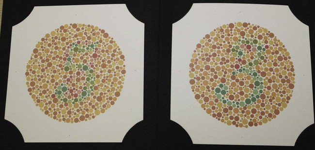
The Ishihara test (Figure 3.7) is a very efficient screening test for red–green colour deficiency and provides quick and simple measurements.41 It is by far the most commonly used colour vision test and is a required entrance test for several professions throughout the world, including the armed forces, aviation and railway industries. Disadvantages include that the Ishihara plates do not assess tritan colour problems. In addition, it is designed as a screening test around the normal/abnormal boundary and is therefore less useful for grading the severity of a defect or for monitoring an acquired colour deficiency. To grade the severity of a congenital or acquired colour deficiency, for monitoring acquired colour defects, and detecting blue–yellow defects, either the City University or Farnsworth D-15 tests or similar tests are recommended. After several years, note that the colours on the Ishihara plates can fade and the test loses its validity. Tests similar to the Ishihara are often provided on computer-based eye examination systems, although their validity has yet to be confirmed.
3.10.2 Procedure: Ishihara test
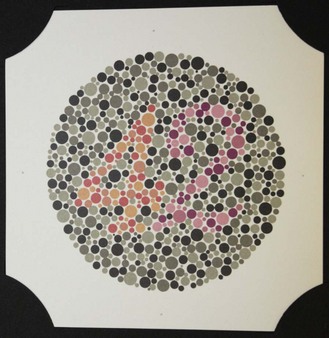
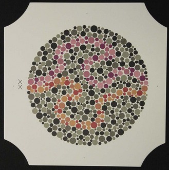
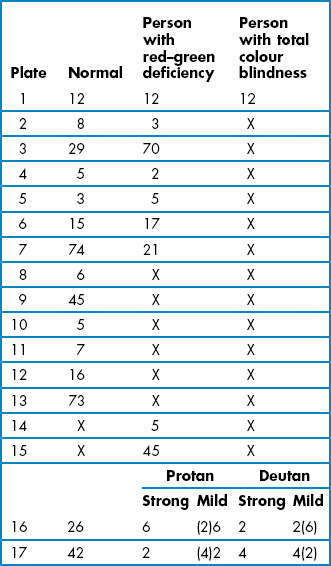
See online video 3.3. The Ishihara test is made up of several plates that present various numbers made up of coloured dots of varying size embedded in a background of different coloured dots (Figure 3.7). The colours of the number and background dots are chosen so that they are confused by patients with red–green colour defects (i.e. they appear isochromatic to those with colour defects) but discriminated by patients with normal colour vision. Plate 1 is a demonstration plate that should be read by all literate patients and can be used to indicate malingerers. Different designs of pseudoisochromatic plates follow, and include transformation (plates 2–9), vanishing (10–17) and hidden digit (18–21) plates. Normal trichromats can see numbers on all but the hidden digit plates. Patients with red–green colour deficiency do not see a number on the vanishing plates, see a different number than normals on the transformation plates (Figure 3.7) and can see a number on the hidden digit plates. Classification plates, which attempt to differentiate protans and deutans, are found on plates 22–25. Two numbers are shown on each plate. The right hand number (blue-purple) is not seen or seen less well by deutans, and the left hand number (red-purple) is not seen or less well seen by protans (Figure 3.8). The rest of the plates contain pseudoisochromatic pathways and are used for patients who cannot read letters, such as young children. The patient’s task is to trace the pathway (Figure 3.9).
1. You must use the proper quantity and quality of illumination, as the colour temperature of the illuminant will affect the colours of the test. Colour vision testing is normally performed under a standard source, such as one of the Gretag Macbeth Sol-Source daylight desk lamps. This simulates natural daylight conditions provided by direct sunlight and a clear sky. As these desk lamps are expensive, alternative sources are also used. For example, you can use high colour rendering fluorescent lights (>5000 K) or a Kodak Wratten #78AA filter (found in camera shops) placed in front of the patient’s eye in conjunction with a 100 watt incandescent light source. Natural daylight is not recommended due to its variability in both the quality and quantity of light, although even this is preferable to tungsten lighting.
2. The Ishihara test (unlike other pseudoisochromatic tests) is insensitive to changes in working distance, duration and blur, so that deviations from the manufacturer’s recommended viewing distance (75 cm) and viewing time (≤3 seconds) do not make a significant difference to errors.42
3. Explain to the patient that you are going to test their colour vision.
4. If screening for a congenital defect, measure colour vision binocularly. If screening for an acquired defect, measure colour vision monocularly.
5. Ask the patient to use their near vision correction and hold the booklet at ~75 cm. Tinted spectacle or contact lenses should be avoided.
6. Ask the patient to read the numbers, starting at plate one. The patient should only be allowed about 3 seconds to view each plate.
7. Use the results sheet to keep a count of any errors. Allow patients another attempt if they make mistakes that are NOT the specific mistakes that red–green colour defectives make.
8. If a patient makes three or more errors, use the classification plates and attempt to categorise the colour defect. Two numbers are shown on each plate and if the patient only reads one number or one number is less visible than the other, the patient can be categorised as deutan (blue–purple letter is not seen or is less visible) or protan (red–purple letter is not seen or is less visible).
9. Any patient who is diagnosed as colour defective should be counselled regarding the effects of the modified colour vision on their everyday life and on future career restrictions.
3.10.4 Interpretation
Patients with red–green colour defects will make specific errors as indicated in Table 3.4. Generally, three or more errors constitutes a fail, although entrance requirements for some professions allow no errors.41,43 Some clinicians do not present the hidden-digit plates, which are not very sensitive to colour deficiency, and just present transformation and vanishing plates.41 Mistakes that are NOT the specific mistakes that red–green colour defectives make should be viewed with caution, as they are much less likely to indicate red–green colour deficiency.43
3.10.6 Alternative procedure: Standard Pseudoisochromatic Plates Part 2
The SPP-2 is another very efficient screening test for red–green colour deficiency and has the advantage over the Ishihara in that it can also be used to screen for blue–yellow defects.44,45 Its major disadvantage is that it is not used as a standard entrance requirement for certain professions like the Ishihara test and therefore is less commonly used. Table 3.5 is a modified score sheet for the SPP-2. Place an ‘X’ through the figures on each plate that were missed and record the total number of blue–yellow, red–green and scotopic errors. Asking the patient to identify which number is more distinct when two figures are seen on each page may only be helpful when testing for subtle differences between the two eyes. If the only BY error was on plate 4, then repeat the plate to rule out the error being caused by the patient’s expectation of seeing only one figure. When totalling the errors, ignore any mistakes of ‘2’ on plate 3 and ‘3’ on plate 6. The ‘2’ is very difficult to discern and almost everyone misses it. The ‘3’ is a reference that can be used to compare the visibility of the two numbers on the page. A patient over 60 years of age fails the test if they make two or more errors, a patient less than 20 years of age fails the blue–yellow part of the test with two or more errors. The failure criteria for all other patients is one or more errors. Classifying an error based on a fail on plate 12 can be confusing because the figure can be missed by individuals with either a protan or tritan defect. In this case, errors on other plates should be considered. With other red–green errors, but not blue–yellow, classify the patient as a protan. With no other red–green errors, then the error should be classified as blue–yellow. With acquired defects, both red–green and blue–yellow errors can occur along with failing plate 12 and additional testing should be carried out with either the Farnsworth-Munsell D-15 or the City University (TCU) test.
3.11 Acquired colour vision
Acquired colour defects are normally monocular or unequal in the two eyes, found about equally in males and females, can progress (or regress) and most often involve a loss of blue sensitivity leading to blue–green and yellow–violet discrimination loss accompanied by decreased vision. Acquired defects may be due to the presence of an anomaly involving the ocular media, retina or the visual pathways. The causes of the anomalies can be due to ocular or systemic diseases and disorders, drugs, or toxic substances. In patients with acquired colour deficiencies, their colour problems can get ignored because other aspects of vision, such as visual acuity, contrast sensitivity or visual fields, are reduced and take precedent. Although these latter tests may be more routinely measured in patients with ocular abnormality and may be more important from a diagnostic perspective, colour vision is an important part of the assessment of a patient’s real world vision. Depending on the prognosis for the condition, young patients with an acquired colour defect should be counselled that their condition lessens their chances of joining certain occupations as discussed in section 3.10. Relatively common causes of acquired colour defects in the working population include diabetes and glaucoma. Note that diabetes can cause blue–yellow defects even prior to the appearance of ophthalmoscopically visible retinopathy.46 Patients who acquire a colour vision problem who have already started a career that requires good colour vision should be warned of possible problems. For example, general medical practitioners should be warned of the difficulties in identifying the presence and extent of various coloured clinical signs such as body colour changes, skin rashes, blood in urine, faeces, sputum and vomit and test strips for blood and urine.40 A tritan-type defect occurs with increasing age due to the yellowing of the lens and receptor changes and cataract (particularly nuclear cataract) and age-related maculopathy in particular can lead to more severe colour defects in the elderly population. Hobbies that may be affected by colour defects include art, photography, interior decorating and electronics. The famous impressionist artist, Claude Monet (1840–1926) had great trouble with acquired colour defects due to cataract in his later life.47 Finally, elderly individuals with colour defects should be warned of differentiating tablets based purely on their colour.
3.11.1 Comparison of tests
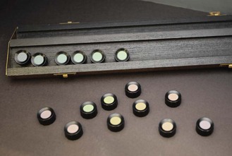
Because the Ishihara test is relatively poor at grading the severity of congenital and acquired colour defects and monitoring acquired colour defects, and cannot detect blue–yellow defects, an additional colour vision test is required. The Farnsworth-Munsell D-15 test consists of 16 caps that each contains a paper of a different colour (Figure 3.10). The differences between the colours are relatively large and the test was designed to separate patients into those with a mild colour defect who pass the test and those with a moderate to severe defect that fail the test. It can grade the severity of colour vision problems and can test for blue–yellow and red–green defects so that it can be used to detect and monitor all patients with acquired colour deficiency. It is more sensitive to protan loss than the City University test.48
The City University test contains ten plates that each displays a central coloured dot surrounded by four coloured dots derived from the Farnsworth-Munsell D-15 test.49 The patient’s task is to select the peripheral coloured dot that looks most similar in colour to the central dot. Three of the peripheral colours are chosen as typical isochromatic confusion colours for patients with a protan, deutan or tritan deficiency respectively. The fourth colour is very similar to the central coloured dot and is the one chosen by patients with normal colour vision. The 2nd edition of the TCU is preferred to the 3rd edition, which has not been independently evaluated and is substantially different from the 2nd edition.49 It can grade the severity of colour vision problems and can test for blue–yellow and red–green defects so that it can be used to detect and monitor all patients with acquired colour deficiency.
3.11.2 Procedure: The Farnsworth-Munsell D-15

1. You must use the proper quantity and quality of illumination as described in 3.10.2, step 1.
2. If grading the severity of a congenital colour vision defect detected using the Ishihara test, measure colour vision binocularly. Explain to the patient that you are going to assess the extent of their colour vision difficulty.
3. If screening for an acquired defect, measure colour vision monocularly. Explain to the patient that you are going to test their colour vision.
4. Ask the patient to use their near vision correction and avoid tinted spectacles or contact lenses.
5. Arrange the loose colour caps in a random order in front of the patient near to the box that contains the pilot colour cap.
6. Ask the patient to place the test cap that most closely resembles the colour of the pilot cap next to it in the box. This then becomes the reference cap for the next test cap, and so on (Figure 3.10) until all caps are in place. Allow the patient time to review the ordering and make any necessary adjustments.
7. Close the box, turn it over and open it again to determine the order that the caps have been arranged.
8. If the caps have been arranged in the correct order, or with just one or two transpositions of adjacent caps, record the result as normal.
9. If mistakes have been made in the arrangement of the caps, record the arrangement order on the D-15 score sheet (Figure 3.11). Draw lines from the numbers on the score sheet according to the patient’s arrangement of the caps. Repeat the test and plot your retest results on a different score sheet (indicate which score relates to which test).
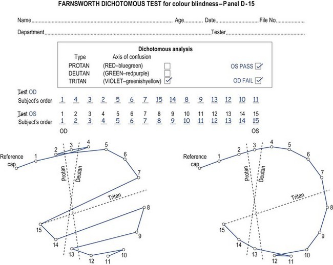
Fig. 3.11 A D-15 scoring sheet showing a tritan defect in the right eye and a passed test in the left eye.
10. Any patients who are diagnosed as colour defective, should be counselled regarding the effects of the modified colour vision on (as appropriate) jobs, hobbies and future career restrictions.
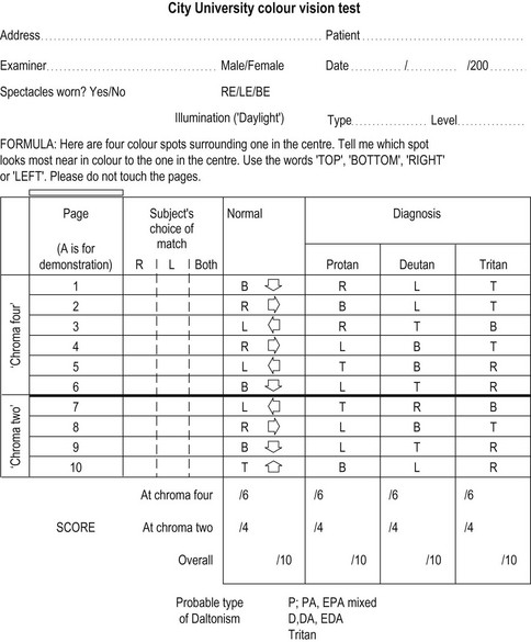
3.11.3 Procedure: The City University (TCU) test
1. You must use the proper quantity and quality of illumination as described in 3.10.2, step 1.
2. If grading the severity of a congenital colour vision defect detected using the Ishihara test, measure colour vision binocularly. Explain to the patient that you are going to assess the extent of their colour vision difficulty.
3. If screening for an acquired defect, measure colour vision monocularly. Explain to the patient that you are going to test their colour vision.
4. Ask the patient to use their near vision correction and avoid tinted spectacles or contact lenses.
5. Hold the test in your hand or place it on the table in front of the patient, about 35 cm away with the pages at right angles to the patient’s line of sight. The cap colours can become soiled with time and some practitioners use white cotton gloves (photographer’s) for themselves and/or the patient.
6. Show the demonstration plate A to the patient and describe the test: ‘Here are four coloured spots surrounding one in the middle. Please tell me which of the four spots is nearest in colour to the one in the middle. Either point or tell me whether it is the top, bottom, left or right, but please don’t touch the pages.’
7. Show the test plates 1 to 10 in turn. Allow about 3 seconds per page, with a slightly longer time for the first few pages while the patient becomes familiar with the task.
8. Record the patient’s choices in the appropriate column on the record card (either right, left or both eyes).
9. Any patients who are diagnosed as colour defective, should be counselled regarding the effects of the modified colour vision on (as appropriate) jobs, hobbies and future career restrictions.
3.11.4 Recording
1. Patients with normal colour vision should make no errors and this can be recorded.
2. The D-15 score sheet should be plotted and retained for patients who make errors. It is also important to record any advice given to the patient and their family.
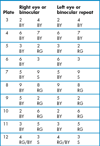
3. The TCU record form (Figure 3.12) indicates the most likely of the four spots which will be called as most similar to the middle by colour normals, protans, deutans and tritans. This can be used to categorise a colour defect in a patient who makes some mistakes. Score the patient’s responses out of 10. The number of mistakes in the normal column indicates the severity of the colour defect. Record if the patient was unusually slow and record any advice given to the patient and their family.
Ishihara failed; D-15 no errors: Mild R/G defect. Patient advised re. effect and future career restrictions.
Ishihara failed; D-15 failed/see attached: mod./severe R/G defect. Patient advised re. effect and future career restrictions.
See attached sheet (Figure 3.11): D-15. OD: Acquired tritan defect. OS: No errors. Fail: patient advised re. possible effect on job as interior decorator.
See attached sheet: TCU. RE: no errors, but slow; OS: 8/10 tritan: Severe acquired tritan defect. Patient advised re. possible effect on job as interior decorator.
3.11.5 Interpretation
Patients with normal colour vision should make no errors.
• D-15: Patients with mild colour vision defects may make minor errors, such as reversals of adjacent caps or one crossing of the D-15 score sheet. These errors still constitute a pass for this test. A failure, as specified by Farnsworth, is two or more crossings of the D-15 score sheet (Figure 3.11). These crossings should parallel one of the protan, deutan or tritan axes marked on the score sheets.
• TCU: A patient ‘fails’ the test if they make more than two mistakes. A patient who makes one or two mistakes is ‘borderline’ and may require retesting or testing with a more extensive battery of tests. The TCU grades the severity and classifies the colour deficiency.49 Patients who fail the Ishihara and then pass the TCU have a mild red–green defect, and are unlikely to have trouble with most occupations.
3.12 Contrast sensitivity
Numerous studies have shown that contrast sensitivity (CS) provides useful information about functional or real-world vision that is not provided by visual acuity, including the likelihood of falling, control of balance, driving, motor vehicle crash involvement, reading, activities of daily living and perceived visual disability.50 It is clear that CS should be included with visual acuity and visual fields in definitions of visual impairment and visual disability and for legal definitions of blindness.51 Thus, using CS in combination with visual acuity (and visual field assessment, when necessary) gives you a better idea of how well a patient actually functions visually. In addition, CS can provide more sensitive measurements of subtle vision loss than visual acuity. There are many clinical situations in which CS can be reduced while VA remains at normal levels, including after refractive surgery, with minimal capsular opacification, with oxidative damage due to heavy smoking, in patients with optic neuritis and multiple sclerosis and in diabetics with little or no background retinopathy.50 For these reasons, CS measurements have become standard for most clinical trials of ophthalmic interventions, and they have been widely used in the assessment of refractive surgery, new intraocular implants, anticataract drug trials and potential treatments for age-related macular degeneration and optic neuritis. CS can therefore be used to help screen for visual pathway disorders and to explain symptoms of poor vision in a patient with good visual acuity. Patients with reduced visual acuity could have normal or reduced CS at low frequencies. Patients with reduced CS will have a poorer quality of vision than those with normal CS, despite the same acuity. When used in combination with visual acuity in this way, CS can be used to help explain symptoms of poor or deteriorating vision and to help justify referral of a cataract patient with reasonable visual acuity. Reduced CS can also explain a poor response to an optical aid by a low vision patient and suggest the need for a contrast enhancing CCTV. Binocular CS that is better than best monocular, can also suggest the desirability of a binocular low vision aid over a monocular one.50
3.12.1 Comparison of tests
Pelli-Robson CS is quickly and simply measured and provides a reliable measurement of low spatial frequency CS (0.5–1 cycles/degree) when measured at the standard 1 m. It provides significantly more repeatable measures than sine-wave grating charts such as the Vistech)52, FACT53 or CSV-1000 charts.54 Other ‘large letter’ contrast sensitivity charts such as the MARS test are similarly repeatable, but those provided on electronic test charts may not be due to issues with liquid crystal display screens at low contrast.55 If high contrast visual acuity is used to assess the high spatial frequency end of the CS curve, then a combination of Pelli-Robson CS and standard VA provides an indication of the whole CS curve. For example, a patient with low frequency CS loss only would have reduced Pelli-Robson CS and normal VA; a patient with high frequency CS loss only would have normal Pelli-Robson CS and reduced VA and a patient with CS loss at all frequencies would have reduced Pelli-Robson CS and reduced VA.50 The Pelli-Robson chart is ideal when determining functional vision loss in patients with low vision and moderate and dense cataract, when screening for low spatial frequency loss in patients with optic neuritis, multiple sclerosis or visual pathway lesions and when examining diabetics with little or no background retinopathy and patients with Parkinson’s or Alzheimer’s disease. The Pelli-Robson chart can be used at longer working distances such as 3 m, so that higher spatial frequencies are assessed and it becomes more sensitive to conditions such as early cataract. One disadvantage of the chart is that a variable endpoint can be gained depending on how long the patient is left to stare at the letters near threshold.50
3.12.2 Procedure
1. Illuminate the chart (Figure 3.13) to between 60 and 120 cd/m2. If room lighting is inadequate, ensure the additional lighting provides a uniform luminance over the chart, and avoids specular reflections from the surface.
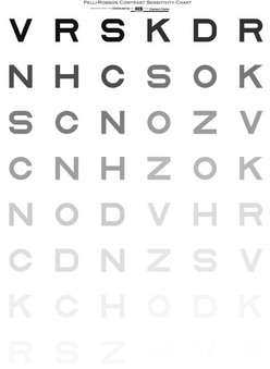
Fig. 3.13 The Pelli-Robson letter contrast sensitivity chart. (Reproduced with permission from Pelli DG, Robson JG and Wilkins AJ. The design of a new letter chart for measuring contrast sensitivity. Clinical Vision Sciences 1988;2:187–99.)
2. Sit/stand the patient 1m from the chart, with the middle of the chart at eye level. Longer distances can be used if required.
3. Patients can wear their own distance spectacles as measurements are relatively immune to moderate dioptric blur.
5. Ask the patient to read the lowest letters that they can see, and encourage the patient to guess. Once the patient states that they cannot see any further, indicate where the next lower contrast triplet is on the chart and ask the patient to keep looking at this point for at least 20 seconds. Generally, if given sufficient time, at least one more triplet of letters will become visible in this manner.
6. Count the reading of the letter C as an O as a correct response to further balance the legibility of the letters.50
7. Score 0.05 log CS for every letter read correctly (the first triplet should be ignored as it has a log CS value of 0.00). This ‘by-letter’ scoring provides a more repeatable and sensitive measurement than the manufacturer’s recommended scoring of the lowest line at which the patient can read two of the three letters.50
8. Repeat the measurements in the other eye and binocularly as required.
3.12.5 Most common errors
1. Not allowing the patient at least 20 seconds for the letters to become visible when the patient is near threshold.
2. Not pushing the patient to guess.
3. Inappropriate use of the occluder so that the patient can see the chart binocularly when monocular measurements are being made.
4. Inappropriate illumination (generally too low or not uniform).
3.12.6 Useful additional techniques: Small letter CS and low contrast VA
Small-letter CS is more sensitive than traditional VA to several clinical conditions, such as early cataract and contact lens oedema and should be ideal when attempting to measure subtle losses of vision such as after refractive surgery.56 CS of very small letters, such as 20/30, correlates very highly with VA and the ideal size for a small-letter test may be about 20/50.57 The measurement procedure is very similar to that for the Pelli-Robson chart.
Low-contrast VA charts measure the smallest letter that can be resolved at a fixed contrast and do not measure CS. It is difficult to state which spatial frequencies the low-contrast letter charts are measuring, because this depends on the VA threshold. If only the large letters at the top of the chart can be seen, the score gives an indication of CS at intermediate spatial frequencies. If a patient can see the small letters at the bottom of the chart, the score gives an indication of higher spatial frequencies. Low-contrast VA scores are believed to indicate the slope of the high-frequency end of the CSF. It has been suggested that they can be used to indicate the CSF when used in combination with a low-frequency or peak CS measure such as the Pelli-Robson chart and a high-contrast VA measurement. The lower the contrast of the acuity charts, the more sensitive they become to subtle vision loss. For example, for detecting subtle vision losses in aviators or subtle changes after refractive surgery, 5–10% charts should be used. For greater losses in vision, such as cataract, even the large letters on these very low contrast charts cannot be seen by some patients, and a higher-contrast chart at about 25% is necessary. As with high contrast VA measurements, charts that follow the Bailey-Lovie (logMAR) design principles should be used and the measurement procedure is the same as for high contrast visual acuity (section 3.2).
3.13 Disability glare
Disability glare tests measure the reduction in a patient’s vision due to a peripheral glare source. Light from the glare source is scattered within the patient’s eye and forward light scatter produces a veiling luminance on the retina that reduces the contrast of the retinal image. In the following clinical conditions in which disability glare can be a problem, the site of increase in light scatter is indicated: corneal oedema (corneal epithelium especially) and opacity, post-refractive surgery (corneal epithelium), cataract (particularly posterior subcapsular cataract), post-cataract surgery (capsular remnants) and retinitis pigmentosa and other retinal disorders leaving a large reflective area on the retina.50 Light scatter within the retina may also be increased in conditions such as macular oedema.
3.13.1 Comparison of tests
For routine optometric practice, disability glare is mainly used to help determine functional vision loss in patients with cataract. In these situations, the amount of intraocular light scatter is large and disability glare is probably best determined by remeasuring visual acuity while directing a glare source, such as a penlight or ophthalmoscope, into the eye. The disadvantage of this technique is the lack of standardisation of the amount of glare light reaching the eye.50 This can be remedied by using a standardised glare source such as the Brightness Acuity Tester (BAT), although this is a relatively expensive instrument for what it provides.52 For more specialised practices, more sensitive measures of disability glare can be obtained using a low contrast VA chart or letter contrast sensitivity chart with a BAT or using a straylight meter.52,58 The latter is sensitive to relatively minor changes in intraocular light scatter, such as in contact lens wearers and pre- and post-refractive surgery.58,59
3.13.2 Procedure: Simple penlight glare test
1. Take the measurements with the patient wearing their own distance vision spectacles or contact lenses. It is difficult to measure disability glare with a trial frame/phoropter because the reduced aperture stops some of the glare light getting into the eye. You should check whether the spectacles or contact lenses are badly scratched as this could cause some disability glare.
2. Perform the test without dilating the pupils, so that the normal pupillary constriction from bright light will occur.
3. Occlude the eye not being tested.
4. Direct the penlight into the patient’s eye from about 30 cm and at an angle of 30° from the eye. Alternatively, the slit-lamp illumination system can be used if it is in an appropriate position relative to the visual acuity chart. This helps to standardise the glare angle and distance of the glare source from the eye.
3.14 Potential vision assessment
Potential vision assessments predict the visual function of the neural system behind cataracts or other media opacities and thus predict the potential vision after cataract or other media opacity surgery. The most common cause of poor visual outcome after cataract surgery is ocular comorbidity and, particularly, age-related macular degeneration. This has led to many patients with cataract and macular degeneration not being offered surgery and there are many low vision patients that have cataract as a secondary diagnosis.14 Whether cataract surgery would be beneficial for these patients is unclear, and depends on whether cataract surgery increases the risk of macular degeneration in the years following surgery or not.60–62 Potential vision testing can contribute to the decision of whether surgical intervention is appropriate. Potential vision testing can also be used in the decision of which eye should be operated on with a patient with bilateral cataract and to provide valuable prognostic information to the patient about the likely outcome of surgery.
3.14.1 Comparison of tests
Although fundus biomicroscopy provides a much clearer view of the retina behind media opacity than direct ophthalmoscopy, subtle maculopathies can still provide inconclusive funduscopic findings. Schein et al. reported that 63% of patients who were predicted by an ophthalmic examination to have visual acuity of 6/12 (20/40, 0.5) or worse after surgery (the level at which cataract surgery is typically deemed ‘unsuccessful’) actually attained a visual acuity of 6/9 or better.63 This suggests that potential vision tests are required in addition to standard clinical tests such as case history information, dilated fundus examination and the swinging flashlight test. Unfortunately, the most commonly used tests, the potential acuity meter (PAM) and the various interferometers, cannot penetrate dense or even moderate cataracts and suggest that potential vision is poor in these cases regardless of the state of the neural system.64 In addition, the interferometers in particular can predict good post-operative vision in patients with certain retinal diseases that is not obtainable.65 The ‘super’ pinhole test is a very simple potential vision test that has provided encouragingly accurate results, superior to the previous standard tests of the PAM and interferometers in moderate cataract.64,66,67 This is simply a pinhole visual acuity test that incorporates adaptations to overcome the loss of light when a VA chart is viewed though a pinhole and cataract.
3.14.2 Procedure: Super pinhole test
1. Measure the potential visual acuity of the ‘poorer’ eye first to avoid a patient memorising the letters seen with the better eye and giving a false visual acuity with the poorer eye. Otherwise, measure VA in the right eye first.
2. Ensure that the patient is wearing their near correction.
3. Explain what measurement you are about to take. For example, ‘this test will help us to estimate the vision you are likely to obtain after cataract surgery’.
4. Instruct the patient: ‘Please cover up your left/right eye with the palm of your hand/this occluder’. If using the patient’s hand, make sure that the palm is being used as otherwise the patient may be able to peek through their fingers. Some clinicians prefer to hold the occluder over the patient’s eye themselves to ensure it is properly occluded.
5. Hold a near VA card at an appropriate distance from the patient and illuminate it with a transilluminator or other bright light source (the Retinal Acuity Meter is a commercially available version of the super pinhole test and provides a brightly transilluminated near card with a multiple pinhole occluder).
6. Give the patient a multiple-pinhole occluder and ask them to move it around until they obtain the best view possible of the near card through one of the pinholes.
7. Ask the patient to read the smallest line (or paragraph) that you can see on the chart.
8. Move the transilluminator to illuminate the text that the patient is reading or attempting to read.
9. Once the patient has reached what they believe is the smallest letters they can see, they should be pushed to determine whether they can see anymore. Use prompts such as ‘Can you see any letters on the next line?’ or ‘Have a guess. It doesn’t matter if you get any wrong’. Also allow the patient to move the multiple pinhole occluder around to see if they can see further down the chart with the pinhole in a different position.
3.14.3 Recording
Record the near VA obtained with the super pinhole test:
| Super PH: | RE: N14 | LE: N12 |
| Super PH: | OD: 0.4M | OS: 0.4M |
| Super PH: | OD: 20/20 | OS: 20/30 |
3.14.4 Interpretation
The near VA obtained with the super pinhole VA gives an indication of the possible near VA after uncomplicated cataract surgery. The test cannot bypass dense cataracts so that in such cases the super pinhole result is likely to be worse than the post-operative VA and just represents the minimum VA that is likely to be obtained after surgery.64 Other results and assessments should be taken into account when considering the likely visual outcome after cataract surgery and these include the patient’s age, indications from the case history and results from a dilated fundus examination and swinging flashlight test. Visual acuity in the pseudophakic eye is another useful indicator for patients undergoing second eye surgery.
3.15 Assessment of macular function
3.15.1 Photostress recovery time
Long lasting after-images (longer than 15 seconds) produced by relatively brief flashes of light are due to photochemical changes in the receptors. Light absorption by rhodopsin (it is assumed that cone photopigments work in a similar fashion, although slightly faster) leads to the separation of the retinal chromophore from opsin. This process is called bleaching as it results in the loss of rhodopsin’s purple colour. While the photopigment is being regenerated, the patient will see an after-image. Photostress recovery time (PSRT) determines the speed at which the photopigment regenerates. Recovery time is solely dependent on the speed of regeneration of the photopigment and is therefore a test of retinal function. It should be independent of other disease within the visual pathway and to some extent will be independent of mild cataract as long as sufficient bleaching light can reach the retina. Only macular disease will cause a prolonged photostress recovery time. The main disadvantage of the test is that there is no standardisation of the procedure. Recovery times are primarily dependent on the brightness of the light and the length of time used, and it is best to obtain your own normal values with your own particular technique and instrumentation.68
3.15.2 Procedure
1. Measure distance visual acuity of both eyes (section 3.2).
2. Ask the patient to remove their spectacles, but keep them in their lap so that they can be quickly put back on again.
3. Occlude the ‘bad’ eye. Hold your direct ophthalmoscope or other bright light source about 2–3 cm away from the patient’s ‘good’ eye. Turn on the light and ask the patient to look directly at the light for exactly 10 sec.
4. After 10 sec, remove the ophthalmoscope, ask the patient to put his or her glasses back on and point to the letters one line larger than the patient’s original visual acuity. Ask the patient to read those letters as quickly as he or she can after the after-image has disappeared.
5. Time how long it takes after removal of the bleaching light for the patient to read at least two-thirds of the letters on the line indicated.
3.15.4 Interpretation
When used with patients with unilateral visual acuity loss, the results are compared between the ‘good’ and the ‘bad’ eye. If the recovery times are similar in the two eyes, then the cause of the poor visual acuity in the ‘bad’ eye is likely to be an optic nerve lesion. If the PSRT is much longer in the bad eye compared to the fellow eye, then the cause of the poor visual acuity is likely retinal. It is generally suggested that any PSRT longer than 50 sec is abnormal, and suggests a macular disease rather than optic nerve abnormality. Of course, recovery times are primarily dependent on the brightness of the light and the length of time used, and it is best to obtain your own normal values with your own particular technique and instrumentation.68
References
1. Bailey, IL, Lovie, JE. New design principles for visual acuity letter charts. Am J Optom Physiol Opt. 1976;53:740–745.
2. Elliott, DB, Yang, KC, Whitaker, D. Visual acuity changes throughout adulthood in normal, healthy eyes: seeing beyond 6/6. Optom Vision Sci. 1995;72:186–191.
3. Lovie-Kitchin, JE. Validity and reliability of visual acuity measurements. Ophthalmic Physiol Opt. 1988;8:363–370.
4. Ferris, FL, Bailey, I. Standardizing the measurement of visual acuity for clinical research studies: Guidelines from the Eye Care Technology Forum. Ophthalmology. 1996;103:181–182.
5. McGraw, PV, Winn, B, Gray, LS, Elliott, DB. Improving the reliability of visual acuity measures in young children. Ophthalmic Physiol Opt. 2000;20:173–184.
6. Carkeet, A. Modeling logMAR visual acuity scores: effects of termination rules and alternative forced-choice options. Optom Vision Sci. 2001;78:529–538.
7. Schulze-Bonsel, K, Feltgen, N, Burau, H, et al. Visual acuities ‘hand motion’ and ‘counting fingers’ can be quantified with the Freiburg visual acuity test. Invest Ophthalmol Vis Sci. 2006;47:1236–1240.
8. McGraw, PV, Winn, B. Glasgow Acuity Cards: a new test for the measurement of letter acuity in children. Ophthalmic Physiol Opt. 1993;13:400–404.
9. Jones, D, Westall, C, Averbeck, K, Adolell, M. Visual acuity assessment: a comparison of two tests for measuring children’s vision. Ophthalmic Physiol Opt. 2003;23:541–546.
10. Bailey, IL, Bullimore, MA, Raasch, TW, Taylor, HR. Clinical grading and the effects of scaling. Invest Ophthalmol Vis Sci. 1991;32:422–432.
11. Bailey IL. Visual acuity. In: Borish’s Clinical refraction. (WJ Benjamin, ed.). 2nd ed. Philadelphia: WB Saunders; 2006.
12. Cacho, I, Dickinson, CM, Smith, HJ, Harper, RA. Clinical impairment measures and reading performance in a large age-related macular degeneration group. Optom Vision Sci. 2010;87:344–349.
13. Millodot, M, Millodot, S. Presbyopia correction and the accommodation in reserve. Ophthalmic Physiol Opt. 1989;9:126–132.
14. Elliott, DB, Trukolo-Ilic, M, Strong, JG, et al. Demographic characteristics of the vision-disabled elderly. Invest Ophthalmol Vis Sci. 1997;38:2566–2575.
15. Latham, K, Tabrett, DR. Guidelines for predicting performance with low vision aids. Optom Vision Sci. 2012;89:1316–1326.
16. Burr, JM, Mowatt, G, Hernández, R, et al. The clinical effectiveness and cost-effectiveness of screening for open angle glaucoma: a systematic review and economic evaluation. Health Technol Assess. 2007;11:1–190.
17. Liu, S, Lam, S, Weinreb, RN, et al. Comparison of standard automated perimetry, frequency-doubling technology perimetry, and short-wavelength automated perimetry for detection of glaucoma. Invest Ophthalmol Vis Sci. 2011;52:7325–7331.
18. Noval, S, Contreras, I, Rebolleda, G, et al. A comparison between Humphrey and frequency doubling perimetry for chiasmal visual field defects. Eur J Ophthalmol. 2005;15:739–745.
19. Artes, PH, Iwase, A, Ohno, Y, et al. Properties of perimetric threshold estimates from full threshold, SITA standard, and SITA fast strategies. Invest Ophthalmol Vis Sci. 2002;43:2654–2659.
20. Hudson, C, Wild, JM, O’Neill, EC. Fatigue effects during a single session of automated static threshold perimetry. Invest Ophthalmol Vis Sci. 1994;35:268–280.
21. Anderson, DR, Patella, VM. Automated static perimetry. CV. St. Louis: Mosby; 1999.
22. Wild, JM, Pacey, IE, O’Neill, EC, Cunliffe, IA. The SITA perimetric threshold algorithms in glaucoma. Invest Ophthalmol Vis Sci. 1999;40:1998–2009.
23. Budenz, DL, Rhee, P, Feuer, WJ, et al. Sensitivity and specificity of the Swedish interactive threshold algorithm for glaucomatous visual field defects. Ophthalmology. 2002;109:1052–1058.
24. Leskea, MC, Heijl, A, Hyman, L, et al. Factors for progression and glaucoma treatment: the Early Manifest Glaucoma Trial. Curr Opin Ophthalmol. 2004;15:102–106.
25. Lalle P. The Humphrey visual field analyzer. In: Primary Care of the Glaucomas (M Fingeret, T Lewis, eds). 2nd ed. New York: McGraw-Hill; 2001. pp. 213–53.
26. Katz, J, Sommer, A. Reliability indices of automated perimetric tests. Arch Ophthalmol. 1988;106:1252–1254.
27. Heijl, A, Lindgren, G, Olsson, J. A package for the statistical analysis of visual fields. Doc Ophthalmol Proc Ser. 1987;49:153–168.
28. Heijl, A, Lindgren, A, Lindgren, G. Test re-test variability in glaucomatous visual fields. Am J Ophthalmol. 1989;108:130–135.
29. Wellings, PC. Detection and recognition of visual field defects resulting from lesions involving the visual pathways. Aust NZ J Ophthalmol. 1989;17:331–335.
30. Drasdo, N, Peaston, WC. Sampling systems for visual field assessment and computerised perimetry. Br J Ophthalmol. 1980;64:705–712.
31. Marmor MF, Kellner U, Lai TY, et al. Revised recommendations on screening for chloroquine and hydroxychloroquine retinopathy. Ophthalmology 2011;118:415-22.
32. Schuchard, RA. Validity and interpretation of Amsler grid reports. Arch Ophthalmol. 1993;111:776–780.
33. Achard, OA, Safran, AB, Duret, FC, Ragama, E. Role of the completion phenomenon in the evaluation of Amsler grid results. Am J Ophthalmol. 1995;120:322–329.
34. Fine, AM, Elman, MJ, Ebert, JE, et al. Earliest symptoms caused by neovascular membranes in the macula. Arch Ophthalmol. 1986;104:513–514.
35. Roper-Hall, MJ. The usefulness of the Amsler chart. Eye. 2006;20:508.
36. Esterman, B. Functional scoring of the binocular field. Ophthalmology. 1982;89:1226–1234.
37. Mandahl, A. Red square test for visual field screening. A sensitive and simple bedside test. Acta Ophthalmol. 1994;72:683–687.
38. Elliott, DB, North, I, Flanagan, J. Confrontation visual field tests. Ophthalmic Physiol Opt. 1997;17:S17–S24.
39. Pandit, RJ, Gales, K, Griffiths, PG. Effectiveness of testing visual fields by confrontation. Lancet. 2001;358(9295):1820.
40. Cole, BL. The handicap of abnormal colour vision. Clin Exp Optom. 2004;87:258–275.
41. Birch, J. Efficiency of the Ishihara test for identifying red–green colour deficiency. Ophthalmic Physiol Opt. 1997;17:403–408.
42. Long, GM, Lyman, BJ, Tuck, JP. Distance, duration and blur effects on the perception of pseudoisochromatic stimuli. Ophthalmic Physiol Opt. 1985;5:185–194.
43. Miyahara, E. Errors reading the Ishihara pseudoisochromatic plates made by observers with normal colour vision. Clin Exp Optom. 2008;91:161–165.
44. Hovis, JK, Cawker, CL, Cranton, D. Comparison of the standard pseudoisochromatic plates–Parts 1 and 2–as screening tests for congenital red-green color vision deficiencies. J Am Optom Assoc. 1996;67:320–326.
45. Vu, BL, Easterbrook, M, Hovis, JK. Detection of color vision defects in chloroquine retinopathy. Ophthalmology. 1999;106:1799–1803.
46. Ismail, GM, Whitaker, D. Early detection of changes in visual function in diabetes mellitus. Ophthalmic Physiol Opt. 1998;18:3–12.
47. Elliott, DB, Skaff, A. Vision of the famous: the artist’s eye. Ophthalmic Physiol Opt. 1993;13:82–90.
48. Oliphant, D, Hovis, JK. Comparison of the D-15 and City University (second) color vision tests. Vision Res. 1998;38:3461–3465.
49. Birch, J. Clinical use of the City University Test (2nd edition). Ophthalmic Physiol Opt. 1997;17:466–472.
50. Elliott, DB, Contrast sensitivity and glare testing. In: Borish’s Clinical Refraction (WJ Benjamin, ed.), 2nd ed. Philadelphia: WB Saunders, 2006.
51. Leat, SJ, Legge, GE, Bullimore, MA. What is low vision? A re-evaluation of definitions. Optom Vision Sci. 1999;76:198–211.
52. Elliott, DB, Bullimore, MA. Assessing the reliability, discriminative ability, and validity of disability glare tests. Invest Ophthalmol Vis Sci. 1993;34:108–119.
53. Pesudovs, K, Hazel, CA, Doran, RM, Elliott, DB. The usefulness of Vistech and FACT contrast sensitivity charts for cataract and refractive surgery outcomes research. Br J Ophthalmol. 2004;88:11–16.
54. Kelly, SA, Pang, Y, Klemencic, S. Reliability of the CSV-1000 in adults and children. Optom Vision Sci. 2012;89:1172–1181.
55. Thayaparan, K, Crossland, MD, Rubin, GS. Clinical assessment of two new contrast sensitivity charts. Br J Ophthalmol. 2007;91:749–752.
56. Rabin, J, Wicks, J. Measuring resolution in the contrast domain–the small letter contrast test. Optom Vision Sci. 1996;73:398–403.
57. Elliott, DB, Situ, P. Visual acuity versus letter contrast sensitivity in early cataract. Vision Res. 1998;38:2047–2052.
58. van der Meulen IJ, Engelbrecht LA, van Vliet JM, et al. Straylight measurements in contact lens wear. Cornea 2010;29:516–22.
59. Rozema, JJ, Coeckelbergh, T, van den Berg, TJ, et al. Straylight before and after LASEK in myopia: changes in retinal straylight. Invest Ophthalmol Vis Sci. 2010;51:2800–2804.
60. Casparis, H, Lindsley, K, Kuo, IC, et al. Surgery for cataracts in people with age-related macular degeneration. Cochrane Database Syst Rev. (6):2012.
61. Chakravarthy, U, Wong, TY, Fletcher, A, et al. Clinical risk factors for age-related macular degeneration: a systematic review and meta-analysis. BMC Ophthalmol. 2010;10:31.
62. Wang, JJ, Fong, CS, Rochtchina, E, et al. Risk of age-related macular degeneration 3 years after cataract surgery: paired eye comparisons. Ophthalmology. 2012;119:2298–2303.
63. Schein, OD, Steinberg, EP, Javitt, JC, et al. Variation in cataract surgery practice and clinical outcomes. Ophthalmology. 1994;101:1142–1152.
64. Vianya-Estopa, M, Douthwaite, WA, Funnell, CL, Elliott, DB. Clinician versus potential acuity test predictions of visual outcome after cataract surgery. Optometry. 2009;80:447–453.
65. AHCPR report: Cataract Management Guideline Panel. Cataract in Adults: Management of Real World Impairment. Clinical Practice Guideline, Number 4. Rockville, MD. U.S. Department of Health and Human Services, Public Health Service, Agency for Health Care Policy and Research. AHCPR Pub. No. 93-0542. Feb. 1993.
66. Hofeldt, AJ, Weiss, MJ. Illuminated near card assessment of potential acuity in eyes with cataract. Ophthalmology. 1998;105:1531–1536.
67. Melki, SA, Safar, A, Martin, J, et al. Potential acuity pinhole–A simple method to measure potential visual acuity in patients with cataracts, comparison to potential acuity meter. Ophthalmology. 1999;106:1262–1267.
68. Margrain, TH, Thomson, D. Sources of variability in the clinical photostress test. Ophthalmic Physiol Opt. 2002;22:61–67.