222 Severity-of-Illness Indices and Outcome Prediction
Development and Evaluation
And he will manage the cure best who has foreseen what is to happen from the present state of matters.1
 Background
Predicting outcome is a time-honored duty of physicians, dating back at least to the time of Hippocrates.1 The need for a quantitative approach to outcome prediction, however, is more recent. Although the patient or family members will still want to know the prognosis, there is increasing pressure to measure and publicly report medical care outcomes. In today’s highly competitive healthcare environment, such information may be used to award contracts for care. Information of variable quality2 is readily available on the Internet. The U.S. Department of Health and Human Services maintains a hospital comparison website,3 and comparative information is also available from sites such as www.healthcarechoices.org.4 Local and regional initiatives to assess quality of care are also common. Some “report cards” specifically address the performance of intensive care units (ICUs) by adjusting outcomes using risk stratification systems, so it is essential that the clinician understand the science behind these systems5 and how risk adjustment models may properly be applied. A focus on performance assessment, however, may detract from other potential uses for risk stratification, including more precise risk-benefit decisions, prognostication, resource allocation, efficient assessment of new therapy and technology, and modifications to individual patient management based on severity of illness.
Prognostication based on clinical observation is affected by memory of recent events, inaccurate estimation of the relative contribution of multiple factors, false beliefs, and human limitations such as fatigue.6 An outcome prediction model, on the other hand, will always produce the same estimate from a given dataset and will correctly value the importance of relevant data. In an environment in which clinical judgment may later be reviewed for financial or legal issues, an objective prediction of outcome becomes especially important. Yet, even the best risk stratification tools can generate misleading data when misapplied.7 Discussed in this chapter are the methods by which models are developed, the application of commonly used models in clinical practice, and common reasons why observed outcome may not match predicted outcome in the absence of differences in the quality of care.8
Well-established general methods for stratifying clinical outcomes by the presenting condition of the patient include the ASA Physical Status Classification9 and the Glasgow Coma Scale (GCS).10 ICU-specific systems typically adjust for patient physiology, age, and chronic health condition; and they may also assess admitting diagnosis, location before ICU admission or transfer status, cardiopulmonary resuscitation before admission, surgical status, and use of mechanical ventilation. An ideal approach to comparing outcomes would use variables that characterize a patient’s initial condition, can be statistically and medically related to outcome, are easy to collect, and are independent of treatment decisions.
 Outcome of Interest
Mortality is a commonly chosen outcome because it is easily defined and readily available. Mortality is insufficient as the sole outcome measure, however, because it does not reflect important issues such as return to work, quality of life, or even costs, because early death results in a lower cost than prolonged hospitalization. There is poor correlation between hospital rankings based on death and those based on other complications.7,11 ICU length of stay is difficult to use as a proxy for quality of care, because the frequency of distribution is usually skewed and mean length of stay is always higher than median owing to long-stay outliers.12 Morbidities such as myocardial infarction, prolonged ventilation, stroke or other central nervous system complications, renal failure, and serious infection can be difficult to collect accurately, and administrative records may not reflect all relevant events.8 There is also little standardization on how morbidity should be defined.
Other potential outcomes include ICU or hospital length of stay, resource use, return to work, quality of life, and 1- or 5-year survival. Patient satisfaction is an outcome highly valued by purchasers of health care, but it is subjective13 and requires substantial effort to accomplish successfully.14 Evaluation of ICU performance may require a combination of indicators, including severity of illness and resource utilization.15
 Databases and Definitions
The quality of a risk stratification system depends on the database on which it was developed. Outcome analysis can either be retrospective, relying on existing medical records or administrative databases, or developed prospectively from data collected concurrently with patient care. Retrospective studies using existing data are quicker and less expensive to conduct but may be compromised by missing data,8 imprecise definitions, interobserver variability,16 and changes in medical practice over time.17
Data derived from discharge summaries or insurance claims do not always capture the presence of comorbid disease18 and may be discordant with data that are clinically collected.19 Because some administrative discharge reports truncate the number of reportable events, diagnoses may be missed, and this coding bias is most apparent in severely ill patients.12 Coding errors and use of computer programs to optimize diagnosis-related group reimbursement can also reduce the validity of claims-derived data. Augmentation of administrative data with laboratory values improves model performance.20
A variety of methods can assess the quality of the database, such as reabstraction of a sample of charts by personnel blinded to the initial results and comparison to an independent database. Kappa analysis is a method for quantifying the rate of discrepancies between measurements (values) of the same variable in different databases (i.e., original and reabstracted). A kappa value of 0 represents no (or random) agreement, and 1.0 is perfect agreement, but this statistic must be interpreted in light of the prevalence of the factor being abstracted.21
 Model Development
Once data integrity is ensured, there are a number of possible approaches to relating outcome to presenting condition. The empirical approach is to use a large database and subject the data to a series of statistical manipulations (Box 222-1). Typically, death, a specific morbidity, and resource consumption are chosen as outcomes (dependent variables). Factors (independent variables) thought to affect outcome are then evaluated against a specific outcome using univariate tests (chi-square, Fisher’s exact, or Student t-test) to establish the magnitude and significance of any relationship.
Independent variables should ideally reflect patient condition independent of therapeutic decisions. Measured variables such as “cardiac index” or “hematocrit” are preferred over “use of inotropes” or “transfusion given,” because the criteria for intervention may vary by provider or hospital. Widely used models rely on common measured physiologic variables (heart rate, blood pressure, and neurologic status) and laboratory values (serum creatinine level and white blood cell count). In addition, variables may consider age, physiologic reserve, and chronic health status. Items chosen for inclusion in a scoring system should be readily available and relevant to clinicians involved in the care of these patients, and variables that lack either clinical or statistical bearing on outcome should not be included. This requirement may necessitate specialized scoring systems for patient populations (pediatric, burn and trauma, and possibly acute myocardial infarction patients) exhibiting different characteristics than the general ICU population. For example, left ventricular ejection fraction and reoperative status are important predictors of outcome in the cardiac surgical population but are not routinely measured or not directly relevant to other population groups.22 If the independent variable is dichotomous (yes/no, male/female), a two-by-two table can be constructed to examine the odds ratio and a chi-square test performed to assess significance (Table 222-1). If multiple variables are being considered, the level of significance is generally set smaller than P = .05, using a multiple comparison (e.g., Bonferroni) correction23 to determine a more appropriate P value.
TABLE 222-1 Two-by-Two Contingency Table Examining Relationship of MOF After Open Heart Surgery (Outcome) to a History of CHF (Predictor) in 3830 Patients*
| Predictor Variable: History of CHF | Outcome Variable: MOF | |
|---|---|---|
| YES | NO | |
| Yes | 121 | 846 |
| No | 166 | 2697 |
CHF, congestive heart failure; MOF, multiple organ failure.
* The odds ratio is defined by cross-multiplication (121 × 2697) ÷ (846 × 166). The odds ratio of 2.3 indicates patients with CHF are 2.3 times as likely to develop postoperative organ system failure as those without prior CHF. This univariate relationship can then be tested by chi-square for statistical significance.
Data from Higgins TL, Estafanous FG, Loop FD et al. ICU admission score for predicting morbidity and mortality risk after coronary artery bypass grafting. Ann Thorac Surg 1997;64:1050–8.
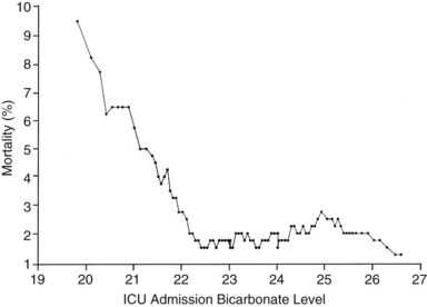
If the independent variable under consideration is a continuous variable (e.g., age) a Student’s t-test is one appropriate choice for statistical comparison. With continuous variables, consideration must be given to the possibility that the relationship of the variable to outcome is not linear. Figure 222-1 demonstrates the relationship of ICU admission serum bicarbonate to mortality outcome in cardiac surgical patients,24 where the data points have been averaged with adjacent values to produce a locally weighted smoothing scatterplot graph.25 Serum bicarbonate values above 22 mmol/L at ICU admission imply a relatively constant risk. Below this value, the risk of death rises sharply. Analysis of this locally weighted smoothing scatterplot graph suggests two ways for dealing with the impact of serum bicarbonate on mortality. One would be to make admission bicarbonate a dichotomous variable (i.e., >22 mEq or <22 mEq). The other would be to transform the data via a logarithmic equation to make the relationship more linear. Cubic splines analysis,26 another statistical smoothing technique, may also be used to assign weight to physiologic variables.
Univariate analysis assesses the forecasting ability of variables without regard to possible correlations or interactions between variables. Linear discriminant and logistic regression techniques can evaluate and correct for overlapping influences on outcome. For example, a history of heart failure and depressed left ventricular ejection fraction are both empirical predictors of poor outcome in patients presenting for cardiac surgery.27 As might be expected, there is considerable overlap between the population with systolic heart failure and those with low ejection fraction. The multivariate analysis in this specific instance eliminates history of heart failure as a variable and retains only measured ejection fraction in the final equation.
Because linear discriminant techniques require certain assumptions about data, logistic techniques are more commonly utilized.4 Subjecting the data to multiple logistic regression will produce an equation with a constant, a β coefficient and standard error, and an odds ratio that represents each term’s effect on outcome. Table 222-2 displays the results of the logistic regression used in the Mortality Probability Model III ICU admission model (MPM0 III). There are 17 variable terms, and a constant term, each with a β value that when multiplied by presence or absence of a factor, becomes part of the calculation of mortality probability using a logistic regression equation. The odds ratios reflect the relative risk of mortality if a factor is present. The challenge in building a model is to include sufficient terms to deliver reliable prediction while keeping the model from being cumbersome to use or too closely fitted to its unique development population. Generally accepted practice is to limit the number of terms in the logistic regression model to 10% of the number of patients having the outcome of interest to avoid “overfitting” the model to the developmental dataset. It is important to identify interaction between variables that may be additive, subtractive (canceling), or synergistic and thus require additional terms in the final model. In the earlier example, seven interaction items were added to reflect important observations in elderly patients,28 who frequently have better outcomes than expected.
TABLE 222-2 Variables in the MPM0 III Logistic Regression Model
| Variable | Odds Ratios (95% Confidence Intervals) | Coefficients (Robust Standard Errors) |
|---|---|---|
| Constant | NA | −5.36283 (0.103) |
| Physiology | ||
| Coma/deep stupor (GCS 3 or 4) | 7.77* (5.921, 10.201) | 2.050514 (0.139) |
| Heart rate ≥150 bpm | 1.54 (1.357,1.753) | 0.433188 (0.065) |
| Systolic BP ≤90 mm Hg | 4.27* (3.393, 5.367) | 1.451005 (0.117) |
| Chronic Diagnoses | ||
| Chronic renal insufficiency | 1.71 (1.580, 1.862) | 0.5395209 (0.042) |
| Cirrhosis | 7.93* (4.820, 13.048) | 2.070695 (0.254) |
| Metastatic neoplasm | 24.65* (15.970, 38.056) | 3.204902 (0.222) |
| Acute Diagnoses | ||
| Acute renal failure | 2.32 (2.137, 2.516) | 0.8412274 (0.042) |
| Cardiac dysrhythmia | 2.28* (1.537, 3.368) | 0.8219612 (0.200) |
| Cerebrovascular incident | 1.51 (1.366, 1.665) | 0.4107686 (0.051) |
| GI bleed | 0.85 (0.763, 0.942) | −0.165253 (0.054) |
| Intracranial mass effect | 6.39* (4.612, 8.864) | 1.855276 (0.166) |
| Other | ||
| Age (per year) | 1.04* (1.037, 1.041) | 0.0385582 (0.001) |
| CPR prior to admission | 4.47* (2.990, 6.681) | 1.497258 (0.205) |
| Mechanical ventilation within 1 hour of admission | 2.27* (2.154, 2.401) | 0.821648 (0.028) |
| Medical or unscheduled surgical admit | 2.48 (2.269, 2.719) | 0.9097936 (0.046) |
| Zero factors (no factors other than age from list above) | 0.65 (0.551, 0.777) | −0.4243604 (0.088) |
| Full code | 0.45 (0.416, 0.489) | −0.7969783(0.041) |
| Interaction Terms | ||
| Age x Coma/deep stupor | 0.99 (0.988,0.997) | −0.0075284 (0.002) |
| Age x Systolic BP ≤ 90 | 0.99 (0.988, 0.995) | −0.0085197 (0.002) |
| Age x Cirrhosis | 0.98 (0.970, 0.986) | −0.0224333 (0.004) |
| Age x Metastatic neoplasm | 0.97 (0.961, 0.974) | −0.0330237 (0.003) |
| Age x Cardiac dysrhythmia | 0.99 (0.985, 0.995) | −0.0101286 (0.003) |
| Age x Intracranial mass effect | 0.98 (0.978, 0.988) | −0.0169215 (0.003) |
| Age x CPR prior to admission | 0.99 (0.983, 0.995) | −0.011214 (0.003) |
Odds ratios for variables with an asterisk (*) are also affected by the associated interaction terms.
CPR, cardiopulmonary resuscitation within 24 hours preceding admission; BP, blood pressure; bpm, beats per minute; GCS, Glasgow Coma Scale; “x” denotes interaction between each pair of variables listed.
Reprinted with permission from Higgins TL, Teres D, Copes WS et al. Assessing contemporary intensive care unit outcome: an updated mortality probability admission model (MPM0-III). Crit Care Med 2007;35:827–35.
The patient’s diagnosis is an important determinant of outcome,17 but conflicting philosophies exist on how disease status should be addressed by a severity adjustment model. One approach is to define principal diagnostic categories and add a weighted term to the logistic regression equation for each illness. This approach acknowledges the different impact of physiologic derangement by diagnosis. For example, patients with diabetic ketoacidosis have markedly altered physiology but a low expected mortality; a patient with an expanding abdominal aneurysm may show little physiologic abnormality and yet be at high risk for death or morbidity. Too many diagnostic categories, however, may result in too few patients in each category to allow statistical analysis for a typical ICU, and such systems are difficult to use without sophisticated (and often proprietary) software.
The other approach is to ignore disease status and assume that factors such as age, chronic health status, and altered physiology will suffice to explain outcome in large groups of patients. This method avoids issues with inaccurate labeling of illness in patients with multiple problems and the need for lengthy lists of coefficients but could result in a model that is more dependent on having an “average” case mix.29,30 Regardless of the specific approach, age and comorbidities (metastatic or hematologic cancer, immunosuppression, and cirrhosis) are given weight in nearly all ICU models to help account for the patient’s physiologic reserve or ability to recover from acute illness.
 Validation and Testing Model Performance
Models may be validated on an independent dataset or by using the development set with methods such as jackknife or bootstrap validation.31 Two criteria are essential in assessing model performance: calibration and discrimination. Calibration refers to how well the model tracks outcomes across its relevant range. A model may be very good at predicting good outcome in healthy patients and poor outcomes in very sick patients yet unable to distinguish outcome for patients in the middle range. The Hosmer-Lemeshow goodness-of-fit test32 assesses calibration by stratifying the data into categories (usually deciles) of risk. The number of patients with an observed outcome is compared with the number of predicted outcomes at each risk level. If the observed and expected outcomes are very close at each level across the range of the model, the sum of chi-squares will be low, indicating good calibration. The P value for the Hosmer-Lemeshow goodness-of-fit increases with better calibration and should be nonsignificant (i.e., >.05). Special precautions apply to using the Hosmer-Lemeshow tests with very large databases.33
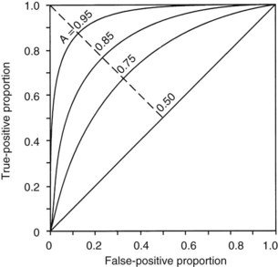
The second measurement of model performance is discrimination, or how well the model predicts the correct outcome. A classification table (Table 222-3) displays four possible outcomes that define sensitivity and specificity of a model with a binary (died/survived) prediction and outcome. Sensitivity (the true-positive rate) and specificity (the true-negative rate, or 1—the false-positive rate) are measures of discrimination but will vary according to the decision point chosen to distinguish between outcomes when a model produces a continuous range of possibilities. The sensitivity and specificity of a model when using 50% as the decision point will differ from that using 95% as the decision point. The classification table can be recalculated for a range of outcomes by choosing various decision points: for example, 10%, 25%, 50%, 75%, and 95% mortality risk. At each decision point, the true-positive rate (proportion of observed deaths predicted correctly) and the false-negative (proportion of survivors incorrectly predicted to die) and overall correct classification rate can be presented. The C-statistic, or area under a receiver-operating characteristic (ROC) curve, is a convenient way to summarize sensitivity and specificity at all possible decision points. A graph of the true-positive proportion (sensitivity) against the false-positive proportion (1—specificity) across the range of the model produces the ROC curve (Figure 222-2). A model with equal probability of producing the correct or incorrect result (e.g., flipping a coin) will produce a straight line at a 45-degree angle that encompasses half of the area (0.5) under the “curve.” Models with better discrimination will incorporate increasingly more area under the curve to a theoretical maximum of 1.0. Most ICU models have ROC areas of 0.8 to 0.9 in the development set, although the ROC area usually decreases when models are applied prospectively to new datasets. The ROC analysis is valid only if the model has first been shown to calibrate well.
| Predicted Outcome | Actual Outcome | |
|---|---|---|
| DIED | SURVIVED | |
| Died | a | c |
| Survived | b | d |
| True-positive ratio = a/(a + b) (sensitivity) | ||
| False-positive ratio = c/(c + d) | ||
| True-negative ratio = d/(c + d) (specificity) | ||
| False-negative ratio = b/(a + b) | ||
| Accuracy (total correct prediction) = (a + d)/a + b + c + d | ||
Adapted from Ruttiman UE. Severity of illness indices: development and evaluation. In: Shoemaker WC, editor. Textbook of critical care medicine. 2nd ed. Philadelphia: Saunders; 1989.
A model may discriminate and calibrate well on its development dataset yet fail when applied to a new population. Discrepancies in performance can relate to differences in surveillance strategies and definitions34 and can occur when a population is skewed by an unusual number of patients having certain risk factors, as could be seen in a specialized ICU.29 Large numbers of low-risk ICU admissions will result in poor predictive accuracy for the entire ICU population.35 The use of sampling techniques (i.e., choosing to collect data randomly on 50% of patients rather than all patients) also appears to bias results.36 Models can also deteriorate over time, owing to changes in populations and medical practice. These explanations should be considered before concluding that quality of care is different between the original and later applications of a model.37
 Standardized Mortality Ratio
Application of a severity-of-illness scoring system involves comparison of observed outcomes with those predicted by the model. The standardized mortality ratio is defined as observed divided by expected mortality and is generally expressed as a mean value ± 95% confidence intervals (CIs), which will depend on the number of patients in the sample. Standardized mortality ratio values of 1.0 (± the CI) indicate that the mortality rate, adjusted for presenting illness, is at the expected level. Standardized mortality ratio values significantly lower than 1.0 indicate performance better than expected. Small differences in scores, as could be caused by consistent errors in scoring elements, timing of data collection, or sampling rate, have been shown to cause important changes in the standardized mortality ratio.36,38
 Models Based on Physiologic Derangement
Three widely utilized general-purpose ICU outcome systems are based on changes in patient physiology: the Acute Physiology and Chronic Health Evaluation (APACHE II,39 APACHE III,40 APACHE IV41), the Mortality Probability Models (MPM I,42 MPM II,43 MPM24,44 MPM0 III45), and the Simplified Acute Physiology Score (SAPS I,46 SAPS II,47 SAPS III48,49). These models are all based on the premise that as illness increases, patients will exhibit greater deviation from physiologic normal for a variety of common parameters such as heart rate, blood pressure, neurologic status, and laboratory values. Risk is also assigned for advanced age and chronic illness.
Acute Physiology and Chronic Health Evaluation
APACHE II was developed from data on 5815 medical and surgical ICU patients at 13 hospitals between 1979 and 1982. Severity of illness was assessed with 12 routine physiologic measurements plus the patient’s age and previous health status.39 Scoring was based on the most abnormal measurements during the first 24 hours in the ICU, and the maximum score is 71 points, although more than 80% of patients have scores of 29 or less.39 Although the developers consider APACHE II to have significant limitations based on its age, it is still in widespread use. APACHE II was developed on a database of medical and surgical patients that excluded patients undergoing coronary artery bypass grafting and coronary care, burn, and pediatric patients. The authors note that “it is crucial to combine the APACHE II score with a precise description of disease” and provide coefficients to adjust the score for 29 nonoperative and 16 postoperative diagnostic categories.39 They also caution that disease-specific mortality predictions be derived from at least 50 patients in each diagnostic category. These appropriate precautions have not always been observed in application of APACHE II.
Another common misunderstanding is to use APACHE II, calibrated for unselected ICU admissions, to assess outcome in a patient sample selected by other criteria, such as severe sepsis. The acute physiology score from APACHE III or a specifically developed model predicting 28-day mortality in sepsis are preferable for risk stratification of septic patients.50 APACHE II does not control for pre-ICU management, which could restore a patient’s altered physiology and lead to a lower score and thus underestimate a patient’s true risk. In a study of 235 medical patients scored with APACHE II, actual mortality was the same as predicted mortality only for patients admitted directly from the emergency department.51 The mortality rate was higher than predicted for transfers from hospital floors, step-down units, or other hospitals. Inclusion of data from the period before ICU admission increases severity of illness scores and thus increases estimated mortality risk, and this effect is greatest with medical patients and emergency admissions.52 Failure to consider the source of admission could thus lead to erroneous conclusions about the quality of medical care.51,52
APACHE III, published in 1991,40 addressed the limitations of APACHE II, including the impact of treatment time and location before ICU admission. The number of separate disease categories was increased from 45 to 78. APACHE III was developed on a representative database of 17,440 patients at 40 hospitals, including 14 tertiary facilities that volunteered for the study and 26 randomly chosen hospitals in the United States. As data accumulated from APACHE III users, the database expanded, and adjustments to coefficients were made to keep data relevant to current practice.17 APACHE III went through several iterations between 1991 and 2003 as part of this continuous updating. Compared with APACHE II, the ranges of physiologic “normal” are narrower with APACHE III and deviations are asymmetrically weighted to be more clinically relevant. Interactions between variables were considered, and five new variables (blood urea nitrogen, urine output, serum albumin, bilirubin, and glucose) were added, and version II variables serum potassium and bicarbonate were dropped. Information was also collected on 34 chronic health conditions, of which 7 (AIDS, hepatic failure, lymphoma, solid tumor with metastasis, leukemia/multiple myeloma, immunocompromised state, and cirrhosis) were significant in predicting outcome.
APACHE III scores range from 0 to 299, and a 5-point increase represents a significant increase in risk of hospital death. In addition to the APACHE III score, which provides an initial risk estimate, there is an APACHE III predictive equation that uses the APACHE III score and proprietary reference data on disease category and treatment location before ICU admission to provide individual risk estimates for ICU patients. Customized models were created for patient populations (e.g., cardiac surgical patients)53 excluded from the APACHE II. Overall correct classification for APACHE III at a 50% cut-point for mortality risk is 88.2%, with an ROC area of 0.90, significantly better than APACHE II.40 Sequential APACHE III scoring can update the risk estimate daily, allowing for real-time decision support, for example, predicting likelihood of ICU interventions over the next 24-hour period. The single most important factor determining daily risk of hospital death is the updated APACHE III score, but the change in the APACHE III score, the admission diagnosis, the age and chronic health status of the patient, and prior treatment are also important. A predicted risk of death in excess of 90% on any of the first 7 days is associated with a 90% mortality rate. APACHE III scores also can be tied to predictions for ICU mortality, length of stay, need for interventions, and nursing workload.
APACHE IV was published in 200641 to address deterioration in APACHE III performance that had developed despite periodic updating over 15 years. APACHE IV has excellent discrimination (ROC area = 0.88) and impressive calibration (Hosmer-Lemeshow C statistic 16.8, P = 0.08) with a sample size of 110,558 patients in the United States. The model includes 142 variables (Table 222-4), many of which were rescaled or revised compared with APACHE III. Using data from 2002-2003 with an observed mortality rate of 13.51, APACHE IV predicted a mortality rate of 13.55, whereas earlier versions of APACHE III predicted 14.64% and 16.90% mortality. A hospital using APACHE III software based on 1988-89 data would have congratulated themselves on a superb SMR of 0.799, where using APACHE IV would have revealed the true SMR to be a respectable but average 0.997, not significantly different than 1.0.
TABLE 222-4 Variables Used in Acute Physiology and Chronic Health Evaluation IV
| Variable | Coefficient | Odds Ratio |
|---|---|---|
| Emergency surgery | 0.2491 | 1.28 |
| Unable to access GCS | 0.7858 | 2.19 |
| Ventilated on ICU day 1 | 0.2718 | 1.31 |
| Thrombolytic therapy for acute myocardial infarction | −0.5799 | 0.56 |
| Rescaled GCS (15-GCS) | 0.0391 | 1.04 |
| 15-GCS = 0 | 1.00 | |
| 15-GCS = 1, 2, 3 | 1.04-1.12 | |
| 15-GCS = 4, 5, 6 | 1.17-1.26 | |
| 15-GCS = 7, 8, 9 | 1.31-1.42 | |
| 15-GCS = 10, 11, 12 | 1.48-1.60 | |
| PaO2/FIO2 ratio: | −0.00040 | 1.00 |
| ≤200 | 1.00-0.92 | |
| 201-300 | 0.92-0.89 | |
| 301-400 | 0.89-0.85 | |
| 401-500 | 0.85-0.82 | |
| 501-600 | 0.82-0.79 | |
| Chronic health items: | ||
| AIDS | 0.9581 | 2.61 |
| Cirrhosis | 0.8147 | 2.26 |
| Hepatic failure | 1.0374 | 2.82 |
| Immunosuppressed | 0.4356 | 1.55 |
| Lymphoma | 0.7435 | 2.10 |
| Myeloma | 0.9693 | 2.64 |
| Metastatic cancer | 1.0864 | 2.96 |
| Admission source: | ||
| Floor | 0.0171 | 1.02 |
| Other hospital | 0.0221 | 1.02 |
| Operating/recovery room | −0.5838 | 0.56 |
AIDS, acquired immunodeficiency syndrome; GCS, Glasgow Coma Scale; ICU intensive care unit.
