Mixing
Andrew M. Twitchell
Chapter contents
Definition and objectives of mixing
Mathematical treatment of the mixing process
Mechanisms of mixing and demixing
Mixing of miscible liquids and suspensions
Key points
Mixing principles
Importance of mixing
There are very few pharmaceutical products that contain only one component. In the vast majority of cases, several ingredients are needed to ensure that the dosage form functions as required. If, for example, a pharmaceutical company wishes to produce a tablet dosage form containing a drug which is active at a dose of 1 mg, other components (e.g. a diluent, binder, disintegrant and lubricant) will be needed both to enable the product to be manufactured and for it to be handled by the patient.
Whenever a product contains more than one component, a mixing or blending stage will be required in the manufacturing process. This may be to ensure an even distribution of the active component(s), an even appearance or that the dosage form releases the drug at the correct site and at the desired rate. The unit operation of mixing is therefore involved at some stage in the production of practically every pharmaceutical preparation and control of mixing processes is of critical importance in assuring the quality of pharmaceutical products. The importance of mixing is illustrated below by the list of products which invariably utilize mixing processes of some kind:
• tablets, capsules, sachets and dry powder inhalers – mixtures of solid particles
• linctuses – mixtures of miscible liquids
Mixing and its control are also important in unit operations such as granulation, drying and coating.
This chapter considers the objectives of the mixing operation, how mixing occurs, and the ways in which a satisfactory mix can be produced and maintained.
Definition and objectives of mixing
Mixing may be defined as a unit operation that aims to treat two or more components, initially in an unmixed or partially mixed state, so that each unit (particle, molecule, etc.) of the components lies as nearly as possible in contact with a unit of each of the other components.
If this is achieved, it produces a theoretical ‘ideal’ situation, i.e. a perfect mix. As will be shown, however, this situation is not normally practicable, is actually unnecessary and, indeed, is sometimes undesirable.
How closely it is attempted to approach the ‘ideal’ situation depends on the product being manufactured and the objective of the mixing operation. For example, when mixing a small amount of a potent drug in a powder mix, the degree of mixing must be of a high order to ensure a consistent dose. Similarly, when dispersing two immiscible liquids or dispersing a solid in a liquid, a well-mixed product is required to ensure product quality/stability. In the case of mixing lubricants with granules during tablet production, however, there is a danger of ‘overmixing’ and the subsequent production of a weak tablet with an increased disintegration time (discussed in Chapter 30).
Types of mixtures
Mixtures may be categorized into three types that differ fundamentally in their behaviour.
Positive mixtures
Positive mixtures are formed from materials such as gases or miscible liquids which mix spontaneously and irreversibly by diffusion and tend to approach a perfect mix. There is no input of energy required with positive mixtures if the time available for mixing is unlimited, although input of energy will shorten the time required to obtain the desired degree of mixing. In general, materials which mix by positive mixing do not present any problems during product manufacture.
Negative mixtures
With negative mixtures, the components will tend to separate out. If this occurs quickly, then energy must be continuously input to keep the components adequately dispersed, e.g. with a suspension formulation where there is a dispersion of solids in a liquid of low viscosity. With other negative mixtures, the components tend to separate very slowly, e.g. emulsions, creams and viscous suspensions. Negative mixtures are generally more difficult to form and to maintain and require a higher degree of mixing efficiency than do positive mixtures.
Neutral mixtures
Neutral mixtures are said to be static in behaviour, i.e. the components have no tendency to mix spontaneously or segregate spontaneously once work has been input to mix them. Examples of this type of mixture include mixed powders, pastes and ointments. Neutral mixes are capable of demixing, but this requires energy input (as discussed in relation to powder segregation later in this chapter).
It should be noted that the type of mixture can change during processing. For example, if the viscosity increases sufficiently, a mixture may change from a negative to a neutral mixture. Similarly, if the particle size, degree of wetting or liquid surface tension changes, the mixture type may also change.
The mixing process
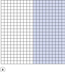
To discuss the principles of the mixing process, a situation will be considered where there are equal quantities of two powdered components of the same size, shape and density that are required to be mixed, the only difference between them being their colour. This situation will not, of course, occur practically but it will serve to simplify the discussion of the mixing process and allow some important considerations to be illustrated with the help of statistical analysis.
If the components are represented by coloured cubes, then a two-dimensional representation of the initial unmixed or completely segregated state can be shown as in Figure 11.1a.
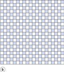
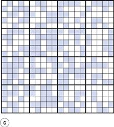
From the definition of mixing, the ideal situation or perfect mix in this case would be produced when each particle lies adjacent to a particle of the other component (i.e. each particle lies as closely as possible in contact with a particle of the other component). This is shown in Figure 11.1b where it can be seen that the components are as evenly distributed as possible. If this mix was viewed in three dimensions then behind and in front of each coloured particle would be a white particle and vice versa. Powder mixing, however, is a ‘chance’ process and while the situation shown in Figure 11.1b could arise, the odds against it are so great that for practical purposes it can be considered impossible. For example, if there are only 200 particles present, the chance of a perfect mix occurring is approximately 1 in 1060 and is similar to the chance of the situation in Figure 11.1a occurring after prolonged mixing. In practice, the best type of mix likely to be obtained will have the components under consideration distributed as indicated in Figure 11.1c. This is referred to as a random mix which can be defined as a mix where the probability of selecting a particular type of particle is the same at all positions in the mix and is equal to the proportion of such particles in the total mix.
If any two adjacent particles are selected from the random mix shown:
• the chance of picking two coloured particles = 1 in 4 (25%)
If any two adjacent particles are selected from the perfect mix shown in Figure 11.1b, there will always be one coloured and one white particle.
Thus if the samples taken from a random mix contain only two particles, then in 25% of cases the sample will contain no white particles and in 25% it will contain no coloured particles. It may help in this and subsequent discussions to imagine the coloured particles as being the active drug and the white particles the inert excipient.
It can be seen that, in practice, the components will not be perfectly evenly distributed, i.e. there will not be full mixing. But if an overall view is taken, the components can be described as being mixed since in the total sample (Fig. 11.1c) the amount of each component is approximately similar (48.8% coloured and 51.2% white). If, however, Figure 11.1c is considered as 16 different blocks of 25 particles, then it can be seen that the number of coloured particles in the blocks varies from six to 19 (24% to 76% of the total number of particles in each block). Careful examination of Figure 11.1c shows that as the number of particles in the sample increases, then the closer will be the proportion of each component to that which would occur with a perfect mix. This is a very important consideration in powder mixing and is discussed in more detail in the following sections.
Scale of scrutiny
Often a mixing process produces a large ‘bulk’ of mixture that is subsequently subdivided into individual dose units (e.g. a tablet, capsule or 5 mL spoonful) and it is important that each dosage unit contains the correct amount/concentration of active component(s). It is the weight/volume of the dosage unit which dictates how closely the mix must be examined/analysed to ensure it contains the correct dose/concentration. This weight/volume is known as the scale of scrutiny and is the amount of material within which the quality of mixing is important. For example, if the unit weight of a tablet is 200 mg then a 200 mg sample from the mix should be analysed to see if mixing is adequate; the scale of scrutiny therefore = 200 mg. If a larger sample size than the scale of scrutiny is analysed this may mask important micro-nonuniformities such as those caused by agglomerates and may lead to the acceptance of an inadequate mix. Conversely, analysing too small a sample size may lead to the rejection of an acceptable mix.
The number of particles contained in the scale of scrutiny will depend on the sample weight, particle size and particle density, and will increase as the sample weight increases and the particle size and density decrease. This number should be sufficient to ensure an acceptably small deviation from the required dose in the dosage forms.
Another important factor to consider when carrying out a mixing process is the proportion of the active component in the dosage form/scale of scrutiny. This is illustrated in Figure 11.2 and in Table 11.1, the latter also demonstrating the importance of the number of particles in the scale of scrutiny.
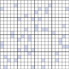
Table 11.1
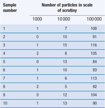
The figures in the table are the numbers of particles of the minor constituent in the samples.
Figure 11.2 shows a random mix containing only 10% coloured particles (active ingredient). If the blocks of 25 particles are examined, it can be seen that the number of coloured particles varies from 0 to 8 or 0% to 32%. Thus, the number of coloured particles as a percentage of the theoretical content varies from 0% to 320%. This is considerably greater than the range of 48 to 152% when the proportion of coloured particles was 0.5 or 50% (Fig. 11.1c).
Table 11.1 shows how the content of a minor (potent) active constituent (present in a proportion of one part in a thousand, i.e. 0.1%) typically varies with the number of particles in the scale of scrutiny, when sampling a random mix. In the example shown, when there are 1000 particles in the scale of scrutiny, three samples contain no active constituent and two have twice the amount that should be present. With 10 000 particles in the scale of scrutiny, the deviation is reduced but samples may still deviate from the theoretical content of 10 particles by ± 50%. Even with 100 000 particles, deviation from theoretical content may be > ± 15% which is generally unacceptable for a pharmaceutical mixture. The difficulty in mixing potent substances can be appreciated if it is realized that there may only be approximately 75 000 particles of diameter 150 µm in a tablet weighing 200 mg.
The information in Figure 11.1, Figure 11.2 and Table 11.1 leads to two important conclusions:
One way of reducing the deviation, therefore, would be to increase the number of particles in the unit dose by decreasing the particle size. This may, however, lead to particle agglomeration due to the increased cohesion and adhesion that occurs with smaller particles, which in turn may reduce the ease of mixing.
It should be noted that with liquid solutions, even very small samples are likely to contain many million ‘particles’. Deviation in content is therefore likely to be very small with miscible liquids even if they are randomly mixed. Diffusion effects in miscible liquids arising from the existence of concentration gradients in an unmixed system mean that they tend to approach a perfect mix.
Mathematical treatment of the mixing process
It should be appreciated that there will always be some variation in the composition of samples taken from a pharmaceutical mix or a random mix. The aim during formulation and processing is to minimize this variation to acceptable levels by selecting an appropriate scale of scrutiny, particle size and mixing procedure (the latter involving the correct choice of mixer, rotation speed, etc.). The following section uses a simplified statistical approach to illustrate some of the factors that influence dose variation within a batch of a dosage form and demonstrates the difficulties encountered with drugs that are active in low doses (potent drugs).
Consider the situation where samples are taken from a random mix in which the particles are all of the same size, shape and density. The variation in the proportion of a component in samples taken from the random mix can be calculated from Equation 11.1:
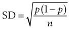 (11.1)
where SD is the standard deviation in the proportion of the component in the samples (content standard deviation), p is the proportion of the component in the total mix and n is the total number of particles in the sample.
Equation 11.1 shows that as the number of particles present in the sample increases, the content standard deviation decreases (i.e. there is less variation in sample content), as illustrated previously by the data in Figure 11.2 and Table 11.1. The situation with respect to the effect of the proportion of the active component in the sample is not as clear from Equation 11.1. As p is decreased, the value of content standard deviation decreases, and this may lead to the incorrect conclusion that it is beneficial to have a low proportion of the active component. A more useful parameter to determine is the percentage coefficient of variation (% CV), which indicates the average deviation as a percentage of the mean amount of active component in the samples. Thus, % CV = (content standard deviation/mean content) × 100. The value of % CV will increase as p decreases, as illustrated in Box 11.1.
Box 11.1 Worked example
Consider the situation where n = 100 000 and p = 0.5. Using Equation 11.1, it can be calculated that the:
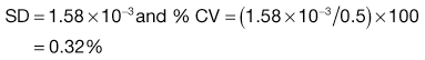
Thus on average, the content will deviate from mean content by 0.32% which is an acceptably low value for a pharmaceutical product.
If, however, p is reduced to 0.001 and n remains at 100 000 there is a reduction in SD to 9.99 × 10⁻⁵ but the

Thus in this latter case, the content will deviate from theoretical content on average by 10% which would be unacceptable for a pharmaceutical product.
It might be considered that the variation in content could be reduced by increasing the unit dose size (increasing the scale of scrutiny), as this would increase the number of particles in each unit dose. The dose of a drug will, however, be fixed and any increase in the unit dose size will cause a reduction in the proportion of the active component in the unit dose. The consequence of increasing the unit dose size depends on the initial proportion of the active component. If p is relatively high initially, increasing the unit dose size causes the %CV in content to increase. If p is small, increasing the unit dose size has little effect. Inserting appropriate values into Equation 11.1 can substantiate this.
In a true random mix the content of samples taken from the mix will follow a normal distribution. With a normal distribution, 68.3% of samples will be within ± 1 SD of the overall proportion of the component (p), 95.5% will be within ± 2 SD of p and 99.7% of samples will be within ± 3 SD of p. For example, if p = 0.5 and the standard deviation in content = 0.02, then for 99.7% of samples the proportion of the component will be between 0.44 and 0.56. In other words, if 1000 samples were analysed, 997 samples would contain between 44% and 56% of drug (mean = 50%).
Ideally for a pharmaceutical product the active component should not deviate by more than ± 5% of the mean or specified content, i.e. the acceptable deviation = p × (5/100) or p × 0.05. Note: this is not the same as a standard deviation of 5%.


