Image Processing

Published on 08/03/2015 by admin

Filed under Opthalmology

Last modified 08/03/2015

Print this page

This article have been viewed 1196 times

Chapter 6 Image Processing

Michael Abràmoff, Christine N. Kay

Introduction

In this review, we discuss quantitative approaches to retinal image analysis. Special emphasis is placed on familiarizing the reader with basic concepts in imaging and image analysis. Fundus and optical coherence tomography (OCT) image analysis are reviewed as well as the use of these modalities in providing comprehensive descriptions of retinal morphology and function. We discuss screening-motivated computer-aided detection of retinal lesions as well as translational clinical applications in diagnosis and therapy.

After reading this chapter the reader should be able to understand concepts in retinal image analysis, and critically review the clinical impact of the research in this field.

History of retinal imaging

The optical properties of the eye that allow image formation prevent direct inspection of the retina. Though existence of the red reflex has been known for centuries, special techniques are needed to obtain a focused image of the retina. The first attempt to image the retina, in a cat, was completed by the French physician Jean Mery, who showed that if a live cat is immersed in water, its retinal vessels are visible from the outside.¹ The impracticality of such an approach for humans led to the invention of the principles of the ophthalmoscope in 1823 by Czech scientist Jan Evangelista (frequently spelled Purkinje) and its reinvention in 1845 by Charles Babbage.^2,³ Finally, the ophthalmoscope was reinvented yet again and reported by von Helmholtz in 1851.⁴ Thus, inspection and evaluation of the retina became routine for ophthalmologists, and the first images of the retina (Fig. 6.1) were published by the Dutch ophthalmologist van Trigt in 1853.⁵ The first useful photographic images of the retina, showing blood vessels, were obtained in 1891 by the German ophthalmologist Gerloff.⁶ In 1910, Gullstrand developed the fundus camera, a concept still used to image the retina today⁷; he later received the Nobel Prize for this invention. Because of its safety and cost-effectiveness at documenting retinal abnormalities, fundus imaging has remained the primary method of retinal imaging.

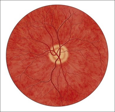
Fig. 6.1 First known image of human retina, as drawn by van Trigt in 1853.

(Reproduced from Trigt AC. Dissertatio ophthalmologica inauguralis de speculo oculi. Utrecht: Universiteit van Utrecht, 1853.)

In 1961, Novotny and Alvis published their findings on fluorescein angiographic imaging.⁸ In this imaging modality, a fundus camera with additional narrow-band filters is used to image a fluorescent dye injected into the bloodstream that binds to leukocytes. It remains widely used, because it allows an understanding of the functional state of the retinal circulation.

The initial approach to depict the three-dimensional (3D) shape of the retina was stereo fundus photography, as first described by Allen in 1964, where multiangle images of the retina are combined by the human observer into a 3D shape.⁹ Subsequently, confocal scanning laser ophthalmoscopy (SLO) was developed, using the confocal aperture to obtain multiple images of the retina at different confocal depths, yielding estimates of 3D shape. However, the optics of the eye limit the depth resolution of confocal imaging to approximately 100 µm, which is poor when compared with the typical 300–500 µm thickness of the whole retina.¹⁰

OCT, first described in 1987 as a method for time-of-flight measurement of the depth of mechanical structures,^11,¹² was later extended to a tissue-imaging technique. This method of determining the position of structures in tissue, described by Huang et al. in 1991,¹³ was termed OCT. In 1993 in vivo retinal OCT was accomplished for the first time.¹⁴ Today, OCT has become a prominent biomedical tissue-imaging technique, especially in the eye, because it is particularly suited to ophthalmic applications and other tissue imaging requiring micrometer resolution.

History of retinal image processing

Matsui et al. were the first to publish a method for retinal image analysis, primarily focused on vessel segmentation.¹⁵ Their approach was based on mathematical morphology and they used digitized slides of fluorescein angiograms of the retina. In the following years, there were several attempts to segment other anatomical structures in the normal eye, all based on digitized slides. The first method to detect and segment abnormal structures was reported in 1984, when Baudoin et al. described an image analysis method for detecting microaneurysms, a characteristic lesion of diabetic retinopathy (DR).¹⁶ Their approach was also based on digitized angiographic images. They detected microaneurysms using a “top-hat” transform, a step-type digital image filter.¹⁷ This method employs a mathematical morphology technique that eliminates the vasculature from a fundus image yet leaves possible microaneurysm candidates untouched. The field dramatically changed in the 1990s with the development of digital retinal imaging and the expansion of digital filter-based image analysis techniques. These developments resulted in an exponential rise in the number of publications, which continues today.

Current status of retinal imaging

Retinal imaging has developed rapidly during the last 160 years and is a now a mainstay of the clinical care and management of patients with retinal as well as systemic diseases. Fundus photography is widely used for population-based, large-scale detection of DR, glaucoma, and age-related macular degeneration. OCT and fluorescein angiography are widely used in the daily management of patients in a retina clinic setting. OCT has also become an increasingly helpful adjunct in preoperative planning and postoperative evaluation of vitreoretinal surgical patients.¹⁸ The overview below is partially based on an earlier review paper.¹⁹

Fundus imaging

We define fundus imaging as the process whereby reflected light is used to obtain a two-dimensional (2D) representation of the 3D, semitransparent, retinal tissues projected on to the imaging plane. Thus, any process that results in a 2D image where the image intensities represent the amount of a reflected quantity of light is fundus imaging. Consequently, OCT imaging is not fundus imaging, while the following modalities/techniques all belong to the broad category of fundus imaging:

1. fundus photography (including so-called red-free photography): image intensities represent the amount of reflected light of a specific waveband

2. color fundus photography: image intensities represent the amount of reflected red (R), green (G), and blue (B) wavebands, as determined by the spectral sensitivity of the sensor

3. stereo fundus photography: image intensities represent the amount of reflected light from two or more different view angles for depth resolution

4. SLO: image intensities represent the amount of reflected single-wavelength laser light obtained in a time sequence

5. adaptive optics SLO: image intensities represent the amount of reflected laser light optically corrected by modeling the aberrations in its wavefront

6. fluorescein angiography and indocyanine angiography: image intensities represent the amounts of emitted photons from the fluorescein or indocyanine green fluorophore that was injected into the subject’s circulation.

There are several technical challenges in fundus imaging. Since the retina is normally not illuminated internally, both external illumination projected into the eye as well as the retinal image projected out of the eye must traverse the pupillary plane. Thus the size of the pupil, usually between 2 and 8 mm in diameter, has been the primary technical challenge in fundus imaging.⁷ Fundus imaging is complicated by the fact that the illumination and imaging beams cannot overlap because such overlap results in corneal and lenticular reflections diminishing or eliminating image contrast. Consequently, separate paths are used in the pupillary plane, resulting in optical apertures on the order of only a few millimeters. Because the resulting imaging setup is technically challenging, fundus imaging historically involved relatively expensive equipment and highly trained ophthalmic photographers. Over the last 10 years or so, there have been several important developments that have made fundus imaging more accessible, resulting in less dependence on such experience and expertise. There has been a shift from film-based to digital image acquisition, and as a consequence the importance of picture archiving and communication systems (PACS) has substantially increased in clinical ophthalmology, also allowing integration with electronic medical records. Requirements for population-based early detection of retinal diseases using fundus imaging have provided the incentive for effective and user-friendly imaging equipment. Operation of fundus cameras by nonophthalmic photographers has become possible due to nonmydriatic imaging, digital imaging with near-infrared focusing, and standardized imaging protocols to increase reproducibility.

Though standard fundus imaging is widely used, it is not suitable for retinal tomography, because of the mixed backscatter caused by the semitransparent retinal layers.

Optical coherence tomography imaging

OCT is a noninvasive optical medical diagnostic imaging modality which enables in vivo cross-sectional tomographic visualization of the internal microstructure in biological systems. OCT is analogous to ultrasound B-mode imaging, except that it measures the echo time delay and magnitude of light rather than sound, therefore achieving unprecedented image resolutions (1–10 µm).²⁰ OCT is an interferometric technique, typically employing near-infrared light. The use of relatively long-wavelength light with a very wide-spectrum range allows OCT to penetrate into the scattering medium and achieve micrometer resolution.

The principle of OCT is based upon low-coherence interferometry, where the backscatter from more outer retinal tissues can be differentiated from that of more inner tissues, because it takes longer for the light to reach the sensor. Because the differences between the most superficial and the deepest layers in the retina are around 300–400 µm, the difference in time of arrival is very small and requires interferometry to measure.²¹

The principle of low coherence, or low correlation, means that the light coming from the light source is only correlating for a short amount of time. In other words, the autocorrelation function of the light wave is only large for a short duration, and at all other times it is essentially zero. If the light is fully coherent, the autocorrelation is high forever, and it becomes impossible to create an interference pattern and determine when the light was emitted; if the light was entirely incoherent, there would be no interference at all. A smaller coherence duration thus results in a better depth resolution, but at lower intensity.

Thus, the low coherence of the light essentially “labels,” with its autocorrelogram, each short duration of the light wave, with the next duration having a different “label.” Though we use the term “label,” it is important to understand that the light wave is actually continuous and not pulsed.

This label uniquely indicates when reflected light was emitted. The low coherent light is optically split into two bundles, called arms, before being sent into the eye. One arm, the reference arm, is aimed at a mirror with a known distance, and thereby reflected; the other, the sample arm, is sent into the eye and reflects back from the different tissues, at yet unknown depth.

If the distance to the mirror is exactly the same as the distance to the tissue, and we optically combine the two reflected (reference and sample) arm light waves, their interference will be nonzero. This is because the more the two light waves resemble each other at a moment in time, the higher the interference; remember that, after splitting, each carried the same low coherence “label.” Because the optical properties of the eye add noise and thus slightly change the reflected reference arm light wave, the interference will never be perfect. Though the coherence pattern or label changes continuously over time, once they are split they have the same “label” (but change rapidly over time), so that the interference will be high as long as the reference and sample distances stay the same. The energy or envelope of the interferogram is measured as intensity at the sensor and is then displayed as the OCT signal intensity. Of course, by changing the position of the mirror, we can “interrogate” the amount of interference at different sample tissue depths.

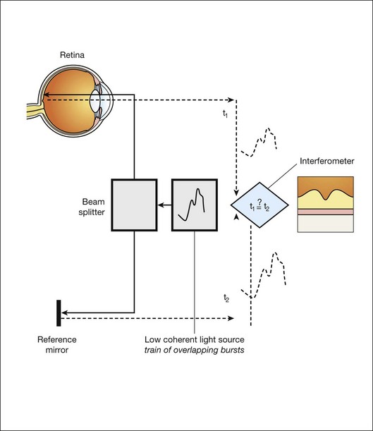
We see the importance of the choice of a good low-coherence source – with either an incoherent or fully coherent source, interferometry is impossible. Such light can be generated by using superluminescent diodes (superbright light-emitting diodes) or lasers with extremely short pulses, femtosecond lasers. The optical setup typically consists of a Michelson interferometer with a low-coherence, broad-bandwidth light source (Fig. 6.2). By scanning the mirror in the reference arm, as in time domain OCT, modulating the light source, as in swept source OCT, or decomposing the signal from a broadband source into spectral components, as in spectral domain OCT (SD-OCT), a reflectivity profile of the sample can be obtained, as measured by the interferogram. The reflectivity profile, called an A-scan, contains information about the spatial dimensions and location of structures within the retina. A cross-sectional tomograph (B-scan) may be achieved by laterally combining a series of these axial depth scans (A-scan). En face imaging (C-scan) at an acquired depth is possible depending on the imaging engine used.

Fig. 6.2 Schematic diagram of the operation of an optical coherence tomography instrument, emphasizing splitting of the light in two arms, overlapping train of bursts “labeled” based on their autocorrelogram, and their interference after being reflected from retinal tissue as well as from the reference mirror (assuming the time delays of both paths are equal).

The transverse resolution of OCT scans (x, y) depends on the speed and quality of the galvanic scanning mirrors and the optics of the eye, and is typically 20–40 µm. The resolution of the A-scans along the z direction depends on the coherence of the light source and is currently 4–8 µm in commercially available scanners. Isotropic (or isometric) means that the size of each imaged element, or voxel, is the same in all three dimensions. Current commercially available OCT devices routinely offer voxel sizes of 30 × 30 × 2 µm, achieving isometricity in the x–y plane only. Available SD-OCT scanners are never truly isotropic, because the retinal tissue in each A-scan is sampled at much smaller intervals in depth than are the distances between A- and/or B-scans. The resolution in depth, or what we call the z-dimension, is currently always higher than the resolution in the x–y plane. The primary advantage of x–y isotropic imaging when quantifying properties of the retina is that fewer assumptions have to be made about the tissue between the measured samples, thus potentially leading to more accurate indices of retinal morphology.

Time domain OCT

With time domain OCT, the reference mirror is moved mechanically to different positions, resulting in different flight time delays for the reference arm light. Because the speed at which the mirror can be moved is mechanically limited, only thousands of A-scans can be obtained per second. The envelope of the interferogram determines the intensity at each depth.¹³ The ability to image the retina two-dimensionally and three-dimensionally depends on the number of A-scans that can be acquired over time. Because of motion artifacts such as saccades, safety requirements limiting the amount of light that can be projected on to the retina, and patient comfort, 1–3 seconds per image or volume is essentially the limit of acceptance. Thus, the commercially available time domain OCT, which allowed collecting of up to 400 A-scans per second, has not yet been suitable for 3D imaging.

Frequency domain OCT

In frequency domain OCT, broadband interference is acquired with spectrally separated detectors, either by encoding the optical frequency in time with a spectrally scanning source or with a dispersive detector, like a grating and a linear detector array. The depth scan can be immediately calculated by Fourier transform from the acquired spectra, without movement of the reference arm. This feature improves imaging speed dramatically, while the reduced losses during a single scan improve the signal to noise proportional to the number of detection elements. The parallel detection at multiple-wavelength ranges limits the scanning range, while the full spectral bandwidth sets the axial resolution.

Spectral domain OCT

A broadband light source is used, broader than in time domain OCT, and the interferogram is decomposed spectrally using a diffraction grating and a complementary metal oxide semiconductor or charged couple device linear sensor. The Fourier transform is again applied to the spectral correlogram intensities to determine the depth of each scatter signal.²² With SD-OCT, tens of thousands of A-scans can be acquired each second, and thus true 3D imaging is routinely possible. Consequently, 3D OCT is now in wide clinical use, and has become the standard of care.

Swept source OCT

Instead of moving the reference arm, as with time domain OCT imaging, in swept source OCT the light source is rapidly modulated over its center wavelength, essentially attaching a second label to the light, its wavelength. A photo sensor is used to measure the correlogram for each center wavelength over time. A Fourier transform on the multiwavelength or spectral interferogram is performed to determine the depth of all tissue scatters at the imaged location.²² With swept source OCT, hundreds of thousands of A-scans can be obtained every second, with additional increase in scanning density when acquiring 3D image volumes.

Areas of active research in retinal imaging

Retinal imaging is rapidly evolving and newly completed research findings are quickly translated into clinical use.

Portable, cost-effective fundus imaging

For early detection and screening, the optimal place for positioning fundus cameras is at the point of care: primary care clinics, public venues (e.g., drug stores, shopping malls). Though the transition from film-based to digital fundus imaging has revolutionized the art of fundus imaging and made telemedicine applications feasible, the current cameras are still too bulky, expensive, and may be difficult to use for untrained staff in places lacking ophthalmic imaging expertise. Several groups are attempting to create more cost-effective and easier-to-use handheld fundus cameras, employing a variety of technical approaches.^23,²⁴

Functional imaging

For the patient as well as for the clinician, the outcome of disease management is mainly concerned with the resulting organ function, not its structure. In ophthalmology, current functional testing is mostly subjective and patient-dependent, such as assessing visual acuity and utilizing perimetry, which are all psychophysical metrics. Among more recently developed “objective” techniques, oxymetry is a hyperspectral imaging technique in which multispectral reflectance is used to estimate the concentration of oxygenated and deoxygenated hemoglobin in the retinal tissue.²⁵ The principle allowing the detection of such differences is simple: deoxygenated hemoglobin reflects longer wavelengths better than does oxygenated hemoglobin. Nevertheless, measuring absolute oxygenation levels with reflected light is difficult because of the large variety in retinal reflection across individuals and the variability caused by the imaging process. The retinal reflectance can be modeled by a system of equations, and this system is typically underconstrained if this variability is not accounted for adequately. Increasingly sophisticated reflectance models have been developed to correct for the underlying variability, with some reported success.²⁶ Near-infrared fundus reflectance in response to visual stimuli is another way to determine the retinal function in vivo and has been successful in cats. Initial progress has also been demonstrated in humans.²⁷

Adaptive optics

The optical properties of the normal eye result in a point spread function width approximately the size of a photoreceptor. It is therefore impossible to image individual cells or cell structure using standard fundus cameras because of aberrations in the human optical system. Adaptive optics uses mechanically activated mirrors to correct the wavefront aberrations of the light reflected from the retina, and thus has allowed individual photoreceptors to be imaged in vivo.²⁸ Imaging other cells, especially the clinically highly important ganglion cells, has thus far been unsuccessful in humans.

Longer-wavelength OCT imaging

3D OCT imaging is now the clinical standard of care for several eye diseases. The wavelengths around 840 µm used in currently available devices are optimized for imaging of the retina. Deeper structures, such as the choroidal vessels, which are important for AMD and other choroidal diseases, and the lamina cribrosa, relevant for glaucomatous damage, are not as well depicted. Because longer wavelengths penetrate deeper into the tissue, a major research effort has been undertaken to develop low-coherence swept source lasers with center wavelengths of 1000–1300 µm. Prototypes of these devices are already able to resolve detail in the choroid and lamina cribrosa.²⁹

Clinical applications of retinal imaging

The most obvious example of a retinal screening application is retinal disease detection, in which the patient’s retinas are imaged in a remote telemedicine approach. This scenario typically utilizes easy-to-use, relatively low-cost fundus cameras, automated analyses of the images, and focused reporting of the results. This screening application has spread rapidly over the last few years, and, with the exception of the automated analysis functionality, is one of the most successful examples of telemedicine.³⁰ While screening programs exist for detection of glaucoma, age-related macular degeneration, and retinopathy of prematurity, the most important screening application focuses on early detection of DR.

Early detection of diabetic retinopathy

Early detection of DR via population screening associated with timely treatment has been shown to prevent visual loss and blindness in patients with retinal complications of diabetes.^31,³² Almost 50% of people with diabetes in the USA currently do not undergo any form of regular documented dilated eye exam, in spite of guidelines published by the American Diabetes Association, the American Academy of Ophthalmology, and the American Optometric Association.³³ In the UK, a smaller proportion or approximately 20% of diabetics are not regularly evaluated, as a result of an aggressive effort to increase screening for people with diabetes. Blindness and visual loss can be prevented through early detection and timely management. There is widespread consensus that regular early detection of DR via screening is necessary and cost-effective in patients with diabetes.³⁴^–³⁷ Remote digital imaging and ophthalmologist expert reading have been shown to be comparable or superior to an office visit for assessing DR and have been suggested as an approach to make the dilated eye exam available to unserved and underserved populations that do not receive regular exams by eye care providers.^38,³⁹ If all of these underserved populations were to be provided with digital imaging, the annual number of retinal images requiring evaluation would exceed 32 million in the USA alone (approximately 40% of people with diabetes with at least two photographs per eye).^39,⁴⁰ In the next decade, projections for the USA are that the average age will increase, the number of people with diabetes in each age category will increase, and there will be an undersupply of qualified eye care providers, at least in the near term. Several European countries have successfully instigated in their healthcare systems early detection programs for DR using digital photography with reading of the images by human experts. In the UK, 1.7 million people with diabetes were screened for DR in 2007–2008. In the Netherlands, over 30 000 people with diabetes were screened since 2001 in the same period, through an early-detection project called EyeCheck.⁴¹ The US Department of Veterans Affairs has deployed a successful photo screening program through which more than 120 000 veterans were screened in 2008. While the remote imaging followed by human expert diagnosis approach was shown to be successful for a limited number of participants, the current challenge is to make the early detection more accessible by reducing the cost and staffing levels required, while maintaining or improving DR detection performance. This challenge can be met by utilizing computer-assisted or fully automated methods for detection of DR in retinal images.⁴²^–⁴⁴

Early detection of systemic disease from fundus photography

In addition to detecting DR and age-related macular degeneration, it also deserves mention that fundus photography allows certain cardiovascular risk factors to be determined. Such metrics are primarily based on measurement of retinal vessel properties, such as the arterial to venous diameter ratio, and indicate the risk for stroke, hypertension, or myocardial infarct.^45,⁴⁶

Image-guided therapy for retinal diseases with 3D OCT

With the introduction of 3D OCT imaging, the wealth of new information about retinal morphology has enabled its usage for close monitoring of retinal disease status and guidance of retinal therapies. The most obvious example of successful image-guided management in ophthalmology is its use in diabetic macular edema. Currently, OCT imaging is widely used to determine the extent and amount of retinal thickening. More detailed analyses of retinal layer morphology and texture from OCT will allow direct image-based treatment to be guided by computer-supported or automated quantitative analysis. This can be subsequently optimized, allowing a personalized approach to retinal disease treatment to become a reality.

Another highly relevant example of a disease that will benefit from image-guided therapy is exudative age-related macular degeneration. With the advent of the anti-vascular endothelial growth factor (VEGF) agents ranibizumab and bevacizumab, it has become clear that outer retinal and subretinal fluid is the main indicator of a need for anti-VEGF retreatment.⁴⁷^–⁵¹ Several studies are under way to determine whether OCT-based quantification of fluid parameters and affected retinal tissue can help improve the management of patients with anti-VEGF agents.

Image analysis concepts for clinicians

Image analysis is a field that relies heavily on mathematics and physics. The goal of this section is to explain the major clinically relevant concepts and challenges in image analysis, with no use of mathematics or equations. For a detailed explanation of the underlying mathematics, the reader is referred to the appropriate textbooks.⁵²

The retinal image

Retinal image analysis

Image analysis is a process by which meaningful information or measurements can be extracted from digital images, typically by computer algorithms. In ophthalmology, image analysis is primarily used to extract clinically relevant measurements from images of the eye, but also to estimate retinal biomarkers, most commonly from fundus color images and from OCT images. The purpose of this section is to familiarize the reader with the main concepts used in the ophthalmic image analysis literature. Image analysis is best understood as a process consisting of a combination of steps. Not all steps are performed in all image analysis algorithms, and some steps may be explicit as multiple steps in one algorithm and form a combined step in another, different algorithm, but the steps described below are typical.

Common image-processing steps

• Preprocessing: remove variability without losing essential information

• Detection: locate specific structures of interest, or features

• Segmentation: determine precise boundaries of objects

• Registration: find similar regions in two or more images

• Interpretation: output clinically relevant information.

Preprocessing

The purpose of preprocessing is to remove as much variation as possible from the image without losing essential information. There are many sources of variation during image acquisition. Image device manufacturer and type, different sizes of field of view, variations in flash illumination, exposure duration, patient movement, variability in retinal pigmentation or in cornea/lens/vitreous opacities are all examples of variation between images taken for the same purpose. These variations do not contribute to the understanding of the image, but they may alter further image analysis steps.

Preprocessing attempts to eliminate some or all of these sources of variation, as much as possible. A simple example is field of view: by scaling the image, and subtracting unexposed areas of the image, images from different cameras are normalized to a “standard fundus image.” Another example is illumination correction, where the pixel intensity values of underexposed areas are increased, and those of overexposed intensities reduced, so that the pixel intensities fall into a narrower and more predictable range.

There are many parallels between image preprocessing using computers and human retinal image processing in ganglion cells.¹⁹

Detection

The purpose of detection is to locate, typically in a preprocessed image, the specific structures of interest, or features, without yet determining their exact boundaries. Examples of such features can be edges, dark or bright spots, oriented lines, and dark–bright transitions in OCT images. Other terms in use for the concept “structure of interest” are wavelets, textures, or filters. Typically, each individual pixel in the image is examined for the presence of one feature or more, and usually the surrounding area, or context, of each pixel is included in this examination. The examination itself usually involves a mathematical computation of the similarity between prototypes of the feature and each pixel and its surround. Conceptually similar terms used in the image analysis literature resembling similarity computation are “correlation,” “convolution,” “lifting,” “matching,” and “comparison.” Usually a nonlinearity is utilized to convert the similarity estimate into a discrete value, for example, “present” versus “nonpresent.”

The output of the matching process indicates if and where the features were detected in the image. In some image analysis systems, this output is interpreted directly, while in others, a segmentation step (see below) is used to determine the exact boundaries of the object represented by the features.

There are many parallels between the features and the convolution process in digital image analysis, and the filters in the human visual cortex.⁵⁵

Segmentation

The purpose of segmentation is to determine the precise boundaries of objects in the image, when the presence of specific object features has been determined in the detection step. For example, if the ganglion cell layer in an OCT image is detected but still has disjoint boundaries, the segmentation step connects these into a connected boundary. Commonly used segmentation techniques are graph search and dynamic programming, both of which try to find the mathematically best-fitting boundary, given the specific detection output(s). The output of the segmentation step can be used directly for assessment, for example when showing the different layers on a macular OCT scan, or can be the input for an interpretation step.

Registration

The purpose of registration is to find similar regions in two or more images so they can be colocalized. Registration is often used to overlay an angiogram on an OCT image, compare images from the same patient from two different visits, to detect improvement or worsening of the patient’s condition between visits, or mosaicing, where several fundus images are stitched together into one image covering a larger area of the retina. The registration step often utilizes similar functions as the detection step.

Interpretation

Usually, when the preceding steps have been completed an interpretation step is used to output clinically relevant information. If the boundaries of the macular retinal layers have been segmented, interpretation involves calculating the distance between the boundaries, so the user can see the thickness of the different layers at specific locations. These thicknesses can even be compared to a database of normal thicknesses at that same location, so that the output represents how likely it is that the retina is thickened at a specific location. Or, after microaneurysms and exudates have been detected and segmented in multiple images from the same patient, these outputs are combined into the clinically relevant information determining whether the patient has more than minimal DR or not.

Unsupervised and supervised image analysis

The design and development of a retinal image analysis system usually involve the combination of some of the steps as explained above, with specific sizes of features and specific operations used to map the input image into the desired interpretation output. The term “unsupervised” is used to indicate such systems. The term “supervised” is used when the algorithm is improved in stepwise fashion by testing whether additional steps or a choice of different parameters can improve performance. This procedure is also called training. The theoretical disadvantage of using a supervised system with a training set is that the provenance of the different settings may not be clear. However, because all retinal image analysis algorithms undergo some optimization of parameters, by the designer or programmer, before clinical use, this is only a relative, not absolute, difference. Two distinct stages are required for a supervised learning/classification algorithm to function: a training stage, in which the algorithm “statistically learns” to classify correctly from known classifications, and a testing or classification stage in which the algorithm classifies previously unseen images. For proper assessment of supervised classification method functionality, training data and performance testing data sets must be completely separate.⁵²

Pixel feature classification

Pixel feature classification is a machine learning technique that assigns one or more classes to the pixels in an image.^55,⁵⁷ Pixel classification uses multiple pixel features including numeric properties of a pixel and the surroundings of a pixel. Originally, pixel intensity was used as a single feature. More recently, n-dimensional multifeature vectors are utilized, including pixel contrast with the surrounding region and information regarding the pixel’s proximity to an edge. The image is transformed into an n-dimensional feature space and pixels are classified according to their position in space. The resulting hard (categorical) or soft (probabilistic) classification is then used either to assign labels to each pixel (for example “vessel” or “nonvessel” in the case of hard classification), or to construct class-specific likelihood maps (e.g., a vesselness map for soft classification). The number of potential features in the multifeature vector that can be associated with each pixel is essentially infinite. One or more subsets of this infinite set can be considered optimal for classifying the image according to some reference standard. Hundreds of features for a pixel can be calculated in the training stage to cast as wide a net as possible, with algorithmic feature selection steps used to determine the most distinguishing set of features. Extensions of this approach include different approaches to classifying groups of neighboring pixels subsequently by utilizing group properties in some manner, for example cluster feature classification, where the size, shape, and average intensity of the cluster may be used.

Measuring performance of image analysis algorithms

Crucial for the acceptance of image analysis algorithms are evaluations of its performance. Most often performance is compared to human experts, though this raises its own set of issues, as explained below. The agreement between an automatic system and an expert reader may be affected by many influences – system performance may become impaired due to the algorithmic limitations, the imaging protocol, properties of the camera used to acquire the fundus images, and a number of other causes. For example, an imaging protocol that does not allow small lesions to be depicted and thus detected will lead to an artificially overestimated system performance if such small lesions might have been detected with an improved camera or better imaging protocol. Such a system then appears to be performing better than it truly is if human experts and the algorithm both overlook true lesions.

Sensitivity and specificity

The performance of a lesion detection system can be measured by its sensitivity, which is the number of true positives divided by the sum of the total number of (incorrectly missed) false negatives plus the number of (correctly identified) true positives.⁵² System specificity is determined as the number of true negatives divided by the sum of the total number of false positives (incorrectly identified as disease) and true negatives. Sensitivity and specificity assessment both require ground truth, which is represented by location-specific discrete values (0 or 1) of disease presence or absence for each subject in the evaluation set. The location-specific output of an algorithm can also be represented by a discrete number (0 or 1). However, the output of the assessment algorithm is often a continuous value determining the likelihood p of local disease presence, with an associated probability value between 0 and 1. Consequently, the algorithm can be made more specific or more sensitive by setting an operating threshold on this probability value, p.